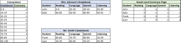
XLOOKUP with Multiple Criteria and Lookup Vector?

[jbiehl]

Hello All!
I'm trying to run an XLOOKUP to create a grade level summary of several different gradebooks based on the student and the subject and convert the values.
A few things need to happen:
1. Pull scores by student for the appropriate subject.
-The subjects will actually be standards and there will be hundreds, so typing the actual subject is not an option.
- It will have to pull from multiple gradebooks. (We won't know if John is in Mrs. Johnson's class or Mr. Smith's class, so it will have to look for him in both classes.)
2. Convert the score bands (listed under the blue) to the corresponding number in the summary.
3. Leave alternating columns untouched.

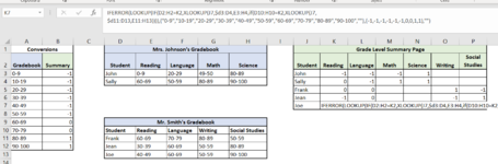
I was thinking something like this might work in K7 for "Joe" but it isn't. IFERROR(LOOKUP(IF(D2:H2=K2,XLOOKUP(J7,$d3:D4,E3:H4,if(D10:H10=K2,XLOOKUP(J7,$d11:D13,E11:H13)))),{"0-9","10-19","20-29","30-39","40-49","50-59","60-69","70-79","80-89","90-100",""},{-1,-1,-1,-1,-1,-1,0,0,1,1),"")

*I am open to the idea of a Query in place of a formula, but I am a Query novice. I'm also not sure if the fact that every other column cannot be changed will make a Query impossible.

Thanks in advance!

 

[ExcelGzh]

jbiehl

If you put this formula
XLOOKUP(IFERROR(INDEX($D:$H,MATCH($J7,$D:$D,0),MATCH(K$2,INDEX($D:$D,XMATCH("Student",INDEX($D:$D,MATCH($J7,$D:$D,0),1):INDEX($D$1,1,1),0,-1),1):INDEX($H:$H,XMATCH("Student",INDEX($D:$D,MATCH($J7,$D:$D,0),1):INDEX($D$1,1,1),0,-1),1),0)),""),$A:$A,$B:$B,"")

into cell K7 and then copy it into the other cells it will do what you want.

It will only work reliably if:
a) Every student's name is unique. It you have duplicate student names you will have to have some other way of uniquely identifying them, say with an ID of some kind.
b) If you extend the Gradebook columns beyond column H you will have to adjust the formula to ensure it still covers all the columns.
c) The word "Student" must appear in the title line of each Grade block.

Brief explanation of what's going on. A Match function requires an array to search in. The result of an Index function is a cell. If you concatenate 2 cells with a colon ":" you create an array, so therefore if you concatenate 2 Index functions with a colon ":" you also create an array. This means you can create the array parameter of a Match function by concatenating 2 Index functions. A simple example is Index(A:A,1,1):Index(A:A,10,1) which is the same as Index(A1:A10). The formula is a series of nested Match functions and concatenated Index functions wrapped up in an Iserror function to trap where the combination of student and subject doesn't exist and then an Xlookup function to find the Summary score.

 

[jbiehl]

jbiehl

If you put this formula
XLOOKUP(IFERROR(INDEX($D:$H,MATCH($J7,$D:$D,0),MATCH(K$2,INDEX($D:$D,XMATCH("Student",INDEX($D:$D,MATCH($J7,$D:$D,0),1):INDEX($D$1,1,1),0,-1),1):INDEX($H:$H,XMATCH("Student",INDEX($D:$D,MATCH($J7,$D:$D,0),1):INDEX($D$1,1,1),0,-1),1),0)),""),$A:$A,$B:$B,"")

into cell K7 and then copy it into the other cells it will do what you want.

It will only work reliably if:
a) Every student's name is unique. It you have duplicate student names you will have to have some other way of uniquely identifying them, say with an ID of some kind.
b) If you extend the Gradebook columns beyond column H you will have to adjust the formula to ensure it still covers all the columns.
c) The word "Student" must appear in the title line of each Grade block.

Brief explanation of what's going on. A Match function requires an array to search in. The result of an Index function is a cell. If you concatenate 2 cells with a colon ":" you create an array, so therefore if you concatenate 2 Index functions with a colon ":" you also create an array. This means you can create the array parameter of a Match function by concatenating 2 Index functions. A simple example is Index(A:A,1,1):Index(A:A,10,1) which is the same as Index(A1:A10). The formula is a series of nested Match functions and concatenated Index functions wrapped up in an Iserror function to trap where the combination of student and subject doesn't exist and then an Xlookup function to find the Summary score.

Thanks for the response and explanation.
This works on the sample sheet. However, in practice, the student rosters are not on the same column. They are actually in separate sheets. How might this formula be adapted to search for students in multiple sheets, instead of just "D:D"? In this example, the students might be found in either Johnson!A:A or Smith!A:A columns.
Thanks again!

 

[ExcelGzh]

jbiehl

If the students were on a different sheet for each teacher then the formula would become very long and convoluted because you would need to repeat the whole thing for each sheet with an error check to deal with when the student wasn't on a particular sheet. Possible with 2 sheets but if you have 5 or 6 or 20 sheets it would be impossible. I think an easier solution would be if you inserted an extra column in the table showing the scores for each student that showed who their teacher was. If you inserted an extra column K and put the teacher's name (which would actually be the name of the sheet) against each student then the formula would look like this:

=XLOOKUP(IFERROR(INDEX(INDIRECT($K3&"!$A:$E"),MATCH($J3,INDIRECT($K3&"!$A:$A"),0),MATCH(L$2,INDEX(INDIRECT($K3&"!$A:$A"),XMATCH("Student",INDEX(INDIRECT($K3&"!$A:$A"),MATCH($J3,INDIRECT($K3&"!$A:$A"),0),1):INDEX(INDIRECT($K3&"!$A$1"),1,1),0,-1),1):INDEX(INDIRECT($K3&"!$E:$E"),XMATCH("Student",INDEX(INDIRECT($K3&"!$A:$A"),MATCH($J3,INDIRECT($K3&"!$A:$A"),0),1):INDEX(INDIRECT($K3&"!$A$1"),1,1),0,-1),1),0)),""),$A:$A,$B:$B,"")

This formula has the INDIRECT function in it and there are a few things to look out for when using INDIRECT. First one is that the cell references inside the quotes, eg "$A:$E", don't update automatically if you change the layout of the sheet the function is looking at. So if you inserted an extra column on the teachers sheets so that the last column became F, you would have to manually change the formula so that every reference to $A:$E became $A:$F.

The second thing to be aware of is that INDIRECT is what they call volatile. This means that it recalculates every time the sheet changes. Usually Excel only recalculates a formula in a particular cell if the calculation decision tree determines that the value in the cell will change because of another change somewhere else on the sheet. This means you can have thousands of formulas but only a handful recalculate if you change a number. With INDIRECT, every formula containing INDIRECT will recalculate regardless of whether the recalculation will produce a different number or not. If you have less than a few hundred INDIRECTs there will be no noticeable change in performance, but if you have thousands of INDIRECTs then there will be a noticeable lag between changing a number and the recalculation completing.

Another thing to be aware of is that if any of your sheet names have spaces in them then the INDIRECT function will need to be modified to include single quotes around the sheet name like this
INDIRECT("'"&$K3&"'!$A:$E"). Fiddly, so it's better to not have spaces in the sheet names, but if you have to have spaces or if other people are going to be using this workbook and they don't know about the no spaces rule then that modification will make it a bit more bullet-proof.