
Compare 3 Lists
August 17, 2017 - by Bill Jelen

You have three lists to compare. Time for lots of VLOOKUP?!
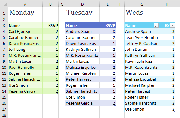
When you think of comparing lists, you probably think of VLOOKUP. If you have two lists to compare, you need to add two columns of VLOOKUP. In the figure below, you are trying to compare Tuesday to Monday and Wednesday to Tuesday and maybe even Wednesday to Monday. It is going to take a lot of VLOOKUP columns to figure out who added and dropped from each list.
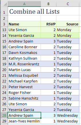
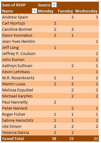
You can use pivot tables to make this job far easier. Combine all of your lists into a single list with a new column called Source. In the Source column, identify which list the data came from. Build a pivot table from the combined list, with Name in ROWS, RSVP in VALUES and Source in COLUMNS. Turn off the Grand Total row and you have a neat list showing a superset from day to day.
Watch Video
- You have three lists to compare. Time for lots of VLOOKUP?!
- There is a far easier way
- Add a "Source" column to the first list and say that list came from List 1
- Copy List 2 beneath List 1
- Copy List 3 to the bottom of both lists
- If you have more lists, keep going
- Create a pivot table from the list
- Move the Source to the columns area
- Remove the grand total
- You now have a superset of items appearing in any list and their answer on each list
- After the credits, a super-fast-motion view of MATCH, VLOOKUP, IFERROR, MATCH, VLOOKUP, IFERROR old way of solving the problem
Video Transcript
Learn Excel for MrExcel Podcast, Episode 2006 -- Compare 3 Lists
Hey, check out this artwork with the chalkboard list. I don't think VLOOKUP would ever work on the chalkboard.
Well it's now September, I've been podcasting this entire book through the entire month of August and we're going to continue in September. Go ahead subscribe to the playlist, top right hand corner.
Hey welcome back to the MrExcel netcast I'm Bill Jelen. We have three lists today. Must be some sort of a party were throwing or maybe a staff meeting. Here's the RSVPs on Monday. Here's the list on Tuesday. Alright so some people are still there Mark Rosenkrantz is there, but some other people have been added and who knows maybe some people have been dropped. It sounds like it's a horrible bunch of VLOOKUPS and not just two VLOOKUPS, three, four. At least four VLOOKUP matches in there, but hey, let's forget about VLOOKUP.
There's an awesome way to do this. That's really, really easy. I'm going to go to the first list and I'm going to add a column called source. Where did this come from? This came from list 1 or in this case, Monday, came from the Monday list and I'm going to take all of the Tuesday data, copy that data, go down to the below list 1 and we will call all this, say that all these records came from Tuesday. And then I'm going to take the Wednesday data, copy that, CTRL C, down to the bottom of the list CTRL V and we'll call it all Wednesday, like this, alright? Then that list, that Superset of all the other lists, and by the way, if I had 4 or 5, 6 lists, I just keep copying them to the bottom. Insert. PivotTable. I'll put it in an existing worksheet. Right here. Okay two click. Okay 5 click okay. Down the left hand side, the name, across the top, Source? and then, whatever we're trying to measure, in this case the number of RSVPs.
Alright, a couple things, let's again Design tab, Report layout, Show in Tabular Form, get real headings up there. We don't need a Grand Total that makes no sense. Right click, remove Grand Total. Alright, we now have a superset of anyone who was in any of the lists. Right, so here Carl had RSVP'd on Monday, but by Tuesday he decided he wasn't coming. So we can see whether we are up or down. Right, this is so much easier than the VLOOKUP method. In fact, if you want to see the VLOOKUP method, wait till after the credits in this video and I'll show you the quick way or a quick look at doing that, but this is the method that's in the book.
Go ahead and buy the book. It's cheap, right? MrExcel XL, 40 greatest excel tips of all time. 25 bucks in print. 10 bucks as an e-book. It has all the information from the August podcast and now the September podcast.
Alright, so you have three lists to compare. Time for lots of VLOOKUP? No, far easier way. Add a source column to the first list and say that those records came from list 1. Copy list 2, beneath list 1. Change the source to say came from list 2. Copy the list 3 to the bottom of both lists. If you have more or less keep going. Create a PivotTable. Source in the columns area; that's the most important part. Remove the Grand Total column and you have a Superset of items appearing in any list and their answer from each list.
Okay, I want to thank you for stopping by, we'll see you next time for another netcast from MrExcel.
Download File
Download the sample file here: Podcast2006.xlsx
Title Photo: Greg Montani / pixabay