Creating the Power Pivot Table

March 21, 2023 - by Bill Jelen

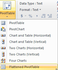
The Pivot Table dropdown offers 8 choices and most of them are fairly silly. PivotTable and Pivot Charts are obviously needed. Pivot table pros will love the Flattened PivotTable. But all of those choices in the middle are redundant. They are trying to tell you that you can combine a pivot table and a chart on the same worksheet. You already know this.

Plus, this menu might make someone think that these are the only options. It is fine to have three charts in a horizontal row and a pivot table vertically below those.

In real life, build your pivot tables and charts one at a time. The first can go on a new worksheet. The others can go on the existing worksheet.

The eighth choice is cool; a flattened pivot table is one where the row labels automatically repeat, and the outer row fields don’t have subtotals. This is great for creating a summary table that will be used for future analysis

Building the Power Pivot Table

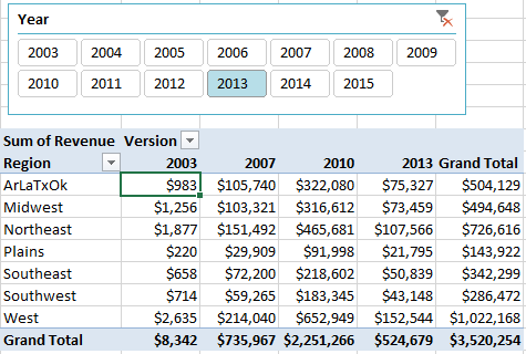
Choose fields from any table and drag them to the four drop zones at the bottom of the field list. Since you’ve created relationships, you are free to use fields from any table.

The pivot table below has region from the Geography table, Excel version from the Product table, Revenue from the Fact table, and a Year slicer from the Date table.

This article is an excerpt from Power Excel With MrExcel

Title photo by Mark Fletcher-Brown on Unsplash