
Date Time to Date
May 15, 2018 - by Bill Jelen

Ian in Nashville gets data every day from a system download. The date column contains Date+Time. This makes the pivot table have multiple rows per day instead of a summary of one cell per day.
This article shows three ways to solve the problem.
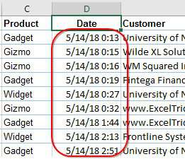
The figure below shows the Date column with Date plus time.
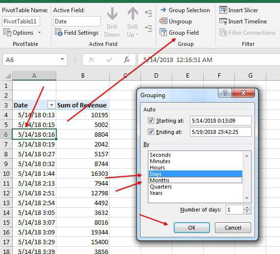
One solution is to fix it in the pivot table.
- Drag the Date field to the Rows area. It shows up with Date+Time.
- Select any cell that contains a date and time.
- On the Pivot Table Tools Analyze tab, choose Group Field.
- In the Grouping dialog, select Days. Unselect Months. When you click OK, the pivot table will show one row per day.
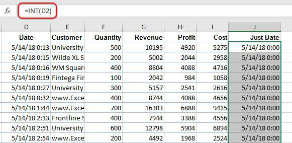
Another tedious solution is to add a new column after the download. As shown in this figure, the formula in column J is =INT(D2).
A date+time is an integer day followed by a decimal time. By using the INT function to get the integer portion of date+time, you isolate the date.
This will work fine, but now you have to add the new column every time you download the data.
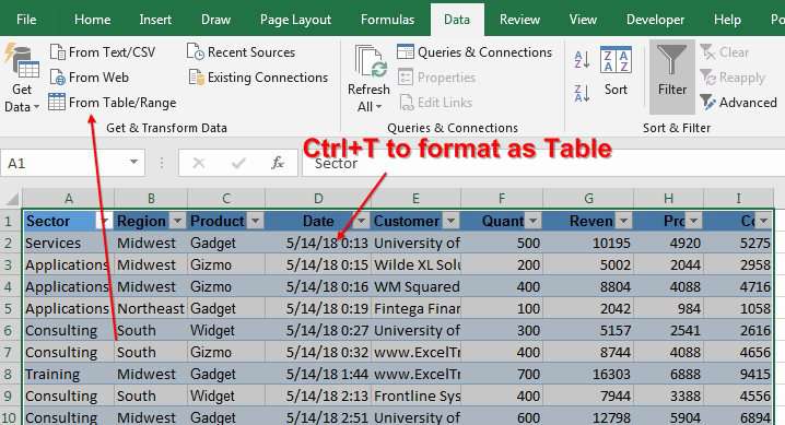
My preferred solution is to use Power Query. Power Query only works in Windows editions of Excel. You can't use Power Query on Android, IOS, or the Mac.
Power Query is built in to Excel 2016. For Excel 2010 and 2013, you can download Power Query from Microsoft.
First, convert the downloaded data to a Table using Ctrl + T. Then, on the Data tab, choose From Table/Range.
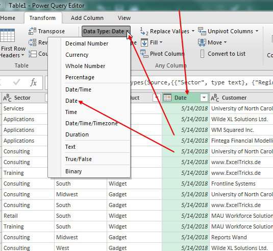
In the Power Query grid, choose the Date column. Go to the Transform tab. Open the Date Type dropdown and choose Date. If you get a message about Replace Step or New Step, choose Replace Step.
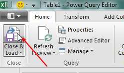
On the Home tab of Power Query, choose Close and Load.
Your result will appear on a new sheet. Create the pivot table from that sheet.
The next time you get new data, follow these steps:
- Paste the new data over the original data set.
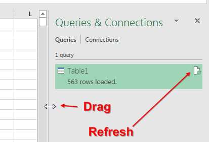
- Go to the sheet with the result of Power Query. Widen the Query panel so you can see Refresh. Click Refresh.
- Refresh the pivot table.
Watch Video
Video Transcript
Learn Excel from MrExcel Podcast, Episode 2203: Truncate Date and Time to Just a Date.
Hey, welcome back to the MrExcel netcast, I'm Bill Jelen. Today's question from Ian in my Nashville Power Excel seminar. Look at this: Ian is getting a download from his system every day, and it has-- in the Date column-- it has Date and Time, and that is screwing things up because when Ian creates a Pivot Table, and puts Dates along the left-hand side, instead of just getting one row per Date, he's getting one row for every Date and Time.
Now, it would be possible to come here and say, Group Field, and group this to Day, click OK. And, you know, that's an extra few clicks that I don't think we have to do. And, so, for this Podcast, the next few Podcasts, we're going to take a look at Power Query. Now, it's built into Excel 2016 here, under Get & Transform Data. If you have 2010 or 2013 running in Windows, not on a Mac, you can download Power Query for free from Excel. And Power Query wants to work on a Table or Range.
So I'm going to choose one cell of data, press Ctrl+T for Table, perfect. And then, on my Power Query tab, Data, From Table/Range, I'm going to choose the Date column and Transform, and say that I want this not to be a Date and Time, but just a Date. I'll choose Replace current, and then Home, Close & Load, and we get a brand new sheet form that has the data converted. Now, from here, of course, we can summarize with a pivot and it'll be perfect.
The advantage, I think, of this method, Power Query, is when Ian gets more data... So here I have new data, I'm going to take this new data, copy the data, and just come here to my old data and paste just below. And, notice that end of table marker right now is in Row 474. When I paste, the end of table marker moves down to the bottom of the new data. Alright? And this query is written based on the table. Alright? So, as the table grows.
Now, one hassle here is, if you're using Power Query for the first time, Power Query starts out that wide-- only half wide-- and you can't see the Refresh icon. So, you have to drag it out here like this and get that great Refresh icon, and just click Refresh. Right now, we have 473 rows loaded, and now 563 rows loaded. Create your pivot table, and life is great.
Now, hey, look, I know it would have been possible to add a new column out here, =INT(D2)-- --of the date-- copy that down, copy and Paste Special Values. But then you're on the hook for doing that every single day. Alright? So while there's at least three different ways we talked about in this video of solving it, for me, Power Query and, just, the ability to click Refresh, is the way to go.
Power Query, I talk about it in my new book, MrExcel LIVe, The 54 Greatest Excel Tips of All Time.
Wrap-up of today's Episode: Ian in Nashville gets data from a system every day, the Date column annoyingly has both Date plus Time-- it screws up his pivot tables, so he has to... Well, three possible things: One, use the INT function, copy, paste values; second, just leave it as Date and Time and then group the pivot table by Date; or, a better solution, Power Query, makes the downloaded data set into a table with Ctrl+T, and then on the Data tab, choose From Table, select the Date and time column, go to the Transform tab in Power Query, convert it to a Date, Close & Load, build the pivot table from that. Next time you get data, paste in the original table, go to the Query panel, click Refresh, and you're good to go.
Hey, to download the workbook from today's video, visit the URL in the YouTube description.
I want to thank Ian for showing up in my seminar in Nashville, I want to thank you for stopping by. I'll see you next time for another netcast from MrExcel.
Download Excel File
To download the excel file: date-time-to-date.xlsx
To further improve the Power Query process:
- Make sure that the download workbook is always saved in the same folder with the same name.
- Start from a blank workbook. Save As with a name like DownloadedFileTransformed.xlsx
- From the blank workbook, Data, From File, From Workbook. Point to the file from Step 1.
- Choose Clean Data. Transform the Date/Time to a Date. Close & Load.
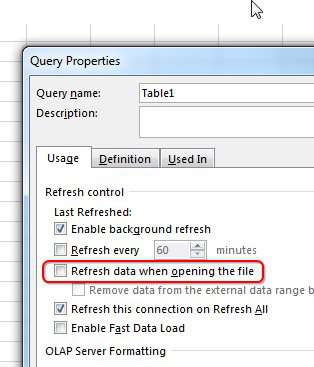
- Right-click the Query Panel and choose Properties. Choose Refresh Data When Opening the File.
- Each day, go to work. Get your coffee. Make sure a new file for #1 is in the folder.
- Open your DownloadFileTransformed.xlsx workbook. It will have the new data and the dates will be correct.
Excel Thought Of the Day
I've asked my Excel Master friends for their advice about Excel. Today's thought to ponder:
"Validation is your friend."
Title Photo: Charisse Kenion on Unsplash