
Dependent Validation Using Arrays
October 18, 2018 - by Bill Jelen

Ever since Data Validation drop-down menus were added to Excel in 1997, people have been trying to work out a way to have the second drop-down menu change based on the selection in the first drop-down.
For example, if you choose Fruit in A2, the drop-down in A4 would offer Apple, Banana, Cherry. But if you choose Herbs from A2, the list in A4 would offer Anise, Basil, Cinnamon. There have been many solutions over the years. I've covered it at least twice in the MrExcel Podcast:
- The classic method used a lot of named ranges as shown in episode 383.
- Another method used OFFSET formulas in Episode 1606.
With the release of the new Dynamic Array formulas in Public Preview, the new FILTER function will give us another way to do Dependent Validation.
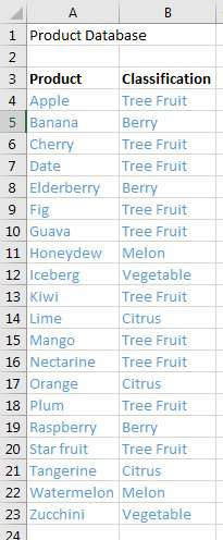
Say that this is your database of products:
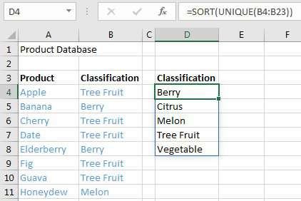
Use a formula of =SORT(UNIQUE(B4:B23)) in D4 to get a unique list of the classifications. This is a brand new type of formula. One formula in D4 returns many answers that will spill into many cells. To refer to the Spiller Range, you would use =D4# instead of =D4.
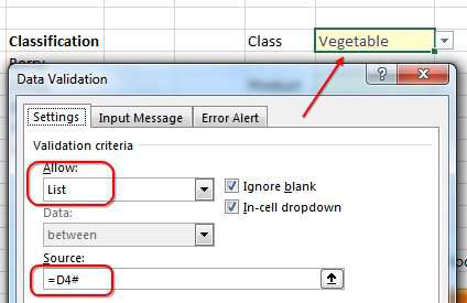
Select a cell to hold the Data Validation menu. Choose Alt+D L to open Data Validation. Change Allow to "List". Specify =D4# as the source of the list. Note that the Hashtag(#) is the Spiller - it means that you are referring to the whole Spiller Range.
The plan is that someone will choose a classification from the first drop-down menu. Then, a formula of =FILTER(A4:A23,B4:B23=H3,"Choose Class First") in E4 will return all of the products in that category. Note that use of "Choose Class First" as the optional third argument. This will prevent a #VALUE! error from appearing.
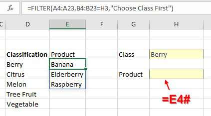
There could be a different number of items in the list depending on the category selected. Setting up Data Validation pointing to =E4# will expand or contract with the length of the list.
Watch Video
Video Transcript
Learn Excel From MrExcel, Podcast Episode 2248: Dependent Validation Using Arrays.
Well, hey. This has been addressed twice before on the podcast, how to do dependent validation, and what dependent validation is is you get to choose, first, a category and then, in response, to that, the second drop-down will change to just the items from that category, and, before, this was complicated, and with the new dynamic arrays that were announced in September of 2018…and these are rolling out, so you have to have Office 365. Right now October 10th, I've heard that they are on about 50% of the Office insiders, so they're rolling them out very slowly. It'll probably be through the first half of 2019 before you get these, but it will allow us to do dependent validation in a much easier fashion.
So, I have two formulas here. The first formula is the UNIQUE of all of the classifications and I sent that into the SORT command. So, that gives me 1 formula returning 5 results and that lives in D4. So, here, where I want to choose the data validation, I'll [DL – 1:09]…the SOURCE is going to be =D4#. That # -- we've been calling it the spiller -- make sure that it returns all of the results from D4. So, if I would add a new category over here and this grows, D4# will pick up that extra amount, alright? [=SORT(UNIQUE(B4:B23))]
So, that first validation is fairly simple, but now that we know that we've chosen CITRUS -- this is going to be more difficult -- I want to filter the list in column A where the item in column B equals the chosen item, alright? So, first we have to let them choose something and then, once I know it's CITRUS, then give me the LIME, ORANGE, and TANGERINE, they would choose something else. BERRY. Check this out. The scientific journals say that a banana is a berry. I don't agree with that. Doesn’t feel like a berry to me but don't blame me. I'm just, you know, using the Internet. BANANA, ELDERBERRY, and RASPBERRY.
Now, you know, the hassle with this is someone's going to initially come here without having chosen anything, and, so in that case, we have CHOOSE CLASS FIRST which is that third argument that says if nothing is found, alright? So, you know, that way, if we start out in this scenario, the choice is going to be CHOOSE CLASS FIRST. The idea is they choose the CLASS, VEGETABLE, this updates, and then those items come from that list. The DATA VALIDATION here, of course, well, that's another spiller, =E4# to get that to work, alright? So, this is cool. (=FILTER(A4:A23,B4:B23=H3,”Choose Class First”)]
Check out my book Excel Dynamic Arrays. This is…it's going to be free through the end of 2018. Check the link down there in the YouTube description, how you can download it, for this very example plus 29 other examples of how to use these items.
Well, wrap up for today. Dynamic arrays give us another way to do dependent validation. If you're not on Office 365 and you don't have these yet, feel free to go back to, I suppose, video 1606 that shows the old way to do this.
I want to thank you for stopping by. We'll see you next time for another netcast from MrExcel.
Download Excel File
To download the excel file: dependent-validation-using-arrays.xlsx
To learn more about Dynamic Arrays, check out Excel Dynamic Arrays Straight To The Point.
Excel Thought Of the Day
I've asked my Excel Master friends for their advice about Excel. Today's thought to ponder:
"Never delete an Excel file without backing it up first."
Title Photo: Félix Prado on Unsplash