
Do All Lookups and Sum the Results
February 09, 2018 - by Bill Jelen

Ron wants to do a bunch of VLOOKUPs and sum the results. There is a single-formula solution to this problem.
Ron asks:
How can you sum all VLOOKUPs without doing each individual lookup?
Many people are familiar with:
=VLOOKUP(B4,Table,2,True)
If you are doing the approximate match version of VLOOKUP (where you specify True as the fourth argument), you can also do LOOKUP.
Lookup is odd because it returns the last column in the table. You don't specify a column number. If your table runs from E4 to J8 and you want the result from column G, you would specify E4:G4 as the lookup table.
Another difference: you don't specify True/False as the fourth argument like you would do in VLOOKUP: the LOOKUP function always does the Approximate Match version of VLOOKUP.
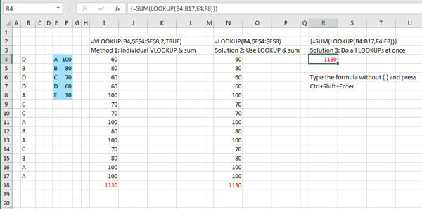
Why bother with this ancient function? Because Lookup has a special trick: You can lookup all of the values at once and it will sum them. Instead of passing a single value such as B4 as the first argument, you can specify all of your values =LOOKUP(B4:B17,E4:F8). Since this would return 14 different values, you have to wrap the function in a wrapper function such as =SUM( LOOKUP(B4:B17,E4:F8)) or =COUNT(LOOKUP(B4:B17,E4:F8)) or =AVERAGE( LOOKUP(B4:B17,E4:F8)). Remember, you need a Wrapper function, but not a rapper function. =SNOOPDOGG(LOOKUP(B4:B17,E4:F8)) won't work.
There is a really common mistake that you will want to avoid. After typing or editing the formula, do not press Enter! Instead, do this three-finger keyboard trick. Hold down Ctrl and Shift. While holding down Ctrl and Shift, press Enter. You can now release Ctrl and Shift. We call this Ctrl + Shift + Enter, but it really has to be timed correctly: Press and hold Ctrl + Shift, Press Enter, Release Ctrl + Shift. If you did it correctly, the formula will appear in the formula bar surrounded by curly braces: {=SUM(LOOKUP(B4:B17,E4:F8))}
Side Note
LOOKUP can also do the equivalent of HLOOKUP. If your lookup table is wider than it is tall, LOOKUP will switch to HLOOKUP. In the case of a tie... a table that is 8x8 or 10x10, LOOKUP will treat the table as vertical.
Watch the video below or study this screenshot.
Watch Video
Video Transcript
Learn Excel from MrExcel Podcast, Episode 2184: Sum All Lookups.
Hey, welcome back to the MrExcel netcast, I'm Bill Jelen. Today's question, from Ron, about using the old, old LOOKUP program. And this is from my book, Excel 2016 In Depth.
Let's say that we had a bunch of products here and we had to use a Lookup table. And for each product, we had to, you know, get the value from the Lookup table and sum that. Well, the typical way is, we use a VLOOKUP-- =VLOOKUP for this product in this table. I'll press F4, lock that down, and with the second value. And in this particular case, because every single value that we're looking up is in the table, and the table is sorted, it's safe to use TRUE. Normally, I would never use TRUE, but in this episode we're going to use TRUE. So I get all of those values and then down here, Alt+=, we get a total of those, right? But what if our whole goal is just to get the 1130? We don't need all these values. We just need this result.
Well, okay, now, there's an old, old function that's been around since the days of Visical, called LOOKUP. Not VLOOKUP. Not HLOOKUP, just LOOKUP. And it seems, at first, similar to be VLOOKUP-- you specify what value you're looking up and the lookup table, press F4, but then we're done. We don't have to specify which column because LOOKUP just goes to the last column in the table. If you had a seven column table and you want to look up the fourth value you would just specify columns one through four. Alright? And, so, whatever the last column is, that's what it's going to look up. And we don't have to specify ,FALSE or ,TRUE because it always uses ,TRUE; there is no ,FALSE version. Alright?
So you have to understand, if you're doing a VLOOKUP, I always use ,FALSE at the end, but in this case it's a short list-- we know that everything in the list is in the table. There's nothing missing, and the table is sorted. Alright? So, this will get us the exact same result that we have for the VLOOKUP.
Awesome, I want to copy this down: Alt+=. Alright. But that doesn't buy us anything because we still have to put all the formulas in and then the SUM function. The beautiful thing is LOOKUP can do a trick that VLOOKUP cannot do, alright? And that is to do all the lookups at once. So, where I send this to the SUM function, when I say LOOKUP, What's the lookup item? We want to lookup all of these things, comma, and then here's the table-- and we don't have to press F4, because we're not going to copy this anywhere, there's only one formula-- close the LOOKUP, close the SUM.
Alright, now, here's the place where things can get screwed up: If you simply press Enter here, you're going to get 60, alright? Because it's just going to go do the first one. What you have to do is hold down the magic three keystrokes, and this is Ctrl+Shift-- I'm holding down Ctrl+shift with my left hand, I keep holding those down, and I press ENTER with my right hand, and it will do all of the math of VLOOKUP. Isn't that awesome? Notice in the formula bar up here, or in the formula text, it puts curly braces around it. You don't type those curly braces, Excel puts those curly braces in, to say, "Hey, you pressed Ctrl+Shift+Enter for this."
Now, hey, this topic and a lot of other topics are in this book: Power Excel with MrExcel, the 2017 edition. Click that "I" up there in the top right-hand corner to read more about the book.
Today, question from Ron: How can you sum all of the VLOOKUPs? Now, most people know the VLOOKUP where you specify the lookup value, the table, which column, and then ,TRUE or ,FALSE. And if you're doing-- if you qualify for-- the TRUE version of VLOOKUP. then you can also do this old LOOKUP. It's odd, because it returns the last column the table, you don't specify column number, and you don't say TRUE or FALSE. It's always TRUE. Why would we use this? Because it has a special trick: You can do all of the lookup values at once and it will sum them. You have to press Ctrl+Shift+Enter after typing that formula or it won't work. And then in the outtake, I'll show you another trick for LOOKUP.
Well, hey, I want to thank Ron for sending that question in, and I want to thank you for stopping by. I'll see you next time for another netcast from MrExcel.
Alright, while we're here talking about LOOKUP, the other thing that LOOKUP can do: You know, we have VLOOKUP for a vertical table like this or HLOOKUP for a horizontal table like this; LOOKUP can go either way. so we can say hey we want to =LOOKUP this value, D, in this table, and because the table is wider than it is tall, LOOKUP automatically switches over to the HLOOKUP version, right? So in this case because we're specifying 3 rows by 5 columns, it will do the HLOOKUP. And because the last row here are the numbers, it will bring us that number. So we have D, Date, gets us 60. Alright. If I would specify a table that only went to row 12, then I will get the name of the product instead. Alright? So it's kind of an interesting little function. I think Excel Help used to say, "Hey, don't use this function," but there's certain times where you can use this function.
Title Photo: grandcanyonstate / pixabay