
Eliminate VLOOKUP with Data Model
August 29, 2017 - by Bill Jelen

Avoid VLOOKUP using the Data Model. So, you have two tables that need joined with VLOOKUP before you can do a pivot table. If you have Excel 2013 or newer on a Windows PC, you can now do this simply and easily.
Say that you have a data set with product, customer, and sales information.
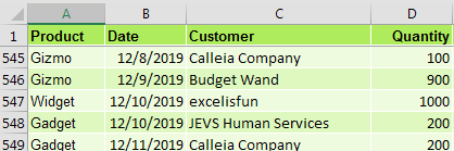
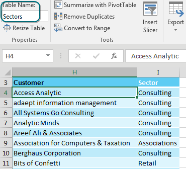
The IT department forgot to put sector in there. Here is a lookup table that maps customer to sector. Time for a VLOOKUP, right?
There is no need to do VLOOKUPs to join these data sets if you have Excel 2013 or Excel 2016. Both of these versions of Excel have incorporated the Power Pivot engine into the core Excel. (You could also do this using the Power Pivot add-in for Excel 2010, but there are a few extra steps.)
In both the original data set and the lookup table, use Home, Format as Table. On the Table Tools tab, rename the table from Table1 to something meaningful. I’ve used Data and Sectors.
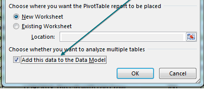
Select one cell in the data table. Choose Insert, Pivot Table. Starting in Excel 2013, there is an extra box Add This Data to the Data Model that you should select before clicking OK.
The Pivot Table Fields list appears with the fields from the Data table. Choose Revenue. Because you are using the Data Model, a new line appears at the top of the list, offering Active or All. Click All.
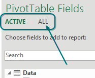
Surprisingly, the PivotTable Fields list offers all the other tables in the workbook. This is groundbreaking. You haven’t done a VLOOKUP yet. Expand the Sectors table and choose Sector. Two things happen to warn you that there is a problem.
First, the pivot table appears with the same number in all the cells.
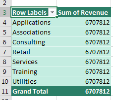
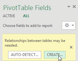
Perhaps the more subtle warning is a yellow box appears at the top of the PivotTable Fields list indicating that you need to create a relationship. Choose Create. (If you are in Excel 2010 or 2016, take your luck with Auto-Detect.)
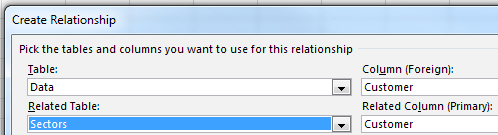
In the Create Relationship dialog, you have four dropdown menus. Choose Data under Table, Customer under Column (Foreign), and Sectors under Related Table. Power Pivot will automatically fill in the matching column under the Related Column (Primary). Click OK.
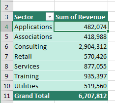
The resulting pivot table is a mashup of the original data and the lookup table. No VLOOKUPs required.
Watch Video
- Starting in Excel 2013, the Pivot Table dialog offers the Data Model
- This is the code word for Power Pivot Engine
- To use the data model, make a Ctrl + T table from each table in the workbook
- Build a pivot table from the first table
- In the Pivot Table Field List, change from Active to All
- Choose a field from the lookup table
- Either create the relationship or Auto-Detect
- Auto-Detect was not there in 2013
- Thanks to Colin Michael and Alejandro Quiceno for suggesting Power Pivot in general.
Video Transcript
Learn Excel from MrExcel podcast, episode 2014 - Eliminate VLOOKUP!
Podcasting this entire book, click the “i” in the top-right hand corner for the playlist!
Hey, welcome back to the MrExcel netcast, I'm Bill Jelen, this is actually called Eliminate VLOOKUP with the Data Model! Now I apologize, this is Excel 2013 and newer, if you're back in Excel 2010, you have to go download the Power Pivot add-in, which of course is free back in 2010. So what we have here is we have our main data set, there's a Customer field here, and then I have a little table that maps customer to sector, I need to create total revenue by sector, right? This is a VLOOKUP, just do a VLOOKUP, but hey, thanks to Excel 2013, we don't have to do a VLOOKUP! I made both of these into a table, and on the Table Tools, Design, I rename the tables, I call this one Sectors, and I call this one Data, to make it into a table, just choose one cell, press Ctrl+T. So if we have some headings and some numbers, when you press Ctrl+T, they ask”Where’s the data for your table?”, My table has headers, and then they call it Table3, you call it something else. Alright, that's how I created those two tables, I'm going to get rid of this table, alright.
So for this trick to work, all the data has to live in tables. We go to the Insert tab, choose PivotTable, and right down here at the bottom, Add this data to the Data Model. This sounds very innocuous, right? There's nothing like flashing point that is saying “Hey, it'll let you do amazing things!” And what they're saying here, what they're trying not to say is that- Oh, by the way, every copy of Excel 2013 has the Power Pivot engine behind it. You know, if you're in Office 365, you're paying $10 a month, and they want you to pay $12 or $15 a month to get Power Pivot, the extra two or five bucks. Well, hey, shh, don't tell, you actually have most of Power Pivot already in Excel 2013. Alright, so I click OK, takes a little bit longer to load the data model, alright, but that's OK, and right over here, in the PivotTable fields, I have a list of all the fields. So, I want to show Revenue, certainly, but what's different is up here with Active and All. When I choose All, I get all the tables in the workbook. Alright, so I go to the Sectors, and I said I want to put sector in the Rows area. Now, initially, the report is going to be wrong, see the 6.7 million all the way down, and this yellow warning over here will say that you have to create a relationship.
Alright now, in 2010 with Power Pivot, it would just, it offered AutoDetect, in 2013 they took AutoDetect out, and in 2016 they brought AutoDetect back, alright? I should show you what CREATE looks like, but when I click this CREATE button, oh yeah, that’s it, alright, good. So from our first table Data, I have a field called Customer, from the related table Sectors, I have a field called Customer, and then you click OK, alright. But let me just show you how cool AutoDetect is, if you happen to be in 2016, there, they figured it out, how awesome is that, right? You don't need to worry about VLOOKUP, and the comma falls at the end, if VLOOKUP makes your head hurt, you're going to love the Data Model. Took those two tables, joined them together, you know, like Access would do, I guess, and created a Pivot table, absolutely amazing. So check the data model next time you have to do a VLOOKUP between two tables. Well this and all the other 40 tips are in the book, Click that “i” on the top-right hand corner. You can buy the book, have a complete cross reference to this entire series of videos, all of August, all of September, heck, we might even carry over into October to get the whole thing done.
Alright, recap today: starting in Excel 2013, the Pivot Table dialog offers something called the Data Model, it's the code word for the Power Pivot engine. Before you create your Pivot tables, do Ctrl+T to make a table from each workbook, I took the extra time to name each one. Build a Pivot table from the first table, and then in the field list, go up to the top and change from Active to All. Choose a field from the lookup table, and then it will warn you that you either have to create a relationship, or AutoDetect, in 2013, you have to click CREATE. But it's what, 4 clicks to create it, 5 if you count the OK button, so really, really easy to do.
Alright, Colin, Michael, and Alejandro Quiceno suggested Power Pivot in general for the books, thanks to them, thanks to you for stopping by, we'll see you next time for another netcast from MrExcel!
Download File
Download the sample file here: Podcast2014.xlsx
Title Photo: LoggaWiggler / pixabay