
Improved Handling of Empty Cells in Pivot Table Source
April 25, 2018 - by Bill Jelen

Quietly and without any fanfare, Microsoft has changed the default behavior for handling empty cells in a pivot table source. In my live Power Excel seminars, when I get to the pivot table section of the day, I can count on at least one person asking me: "Why do my pivot tables default to Count instead of Sum when I drag Revenue to the pivot table." If you have Office 365, a change is coming to Excel to reduce the number of times this happens.
When I get the question, I explain that it is one of two things:
- Is there any chance that you have one or more blank cells in the Revenue column?
- I show that when I create a pivot table, I will select one cell in the source data. But, I know that many people will select the entire column, such as A:I. I appreciate this idea, because if you add more data later, it becomes part of the pivot table with a click of Refresh.
Note
For the people selecting the entire column, I would usually suggest converting their pivot table source data to a table using Ctrl + T. Any data pasted below the table will also become part of the pivot table with a click on Refresh. This was covered in Podcast 2149.
In the past, here is what would happen:
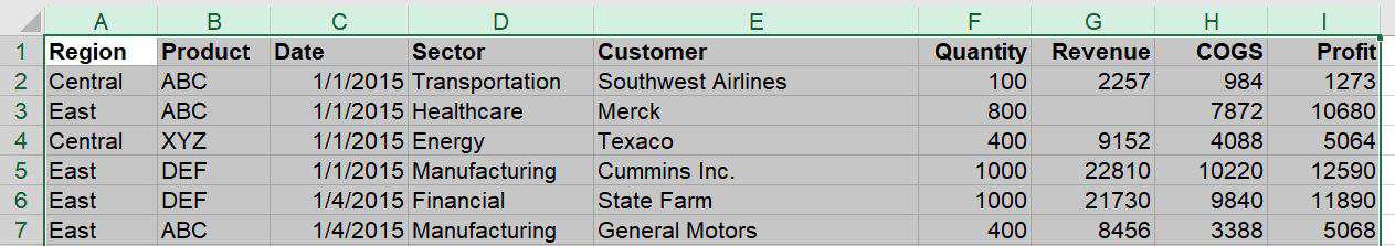
You have a single blank cell in your pivot table data.
In the pivot table field list, if you checkmark Revenue, it will move to the Rows area instead of the Values area. This is rarely what you want.
People who routinely have this problem usually have learned that you want to drag Revenue to the Values area. But this would fail, because now you get a Count instead of a Sum.
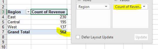
Think about what was happening: A single empty cell in the revenue column will cause a Count instead of Sum. For those people who select A:I instead of A1:I564, you are essentially selecting 563 numeric cells and 1,048,012 blank cells.
The New Improved Feature
The beautiful thing about being an Office 365 subscriber is that the Excel team can push out updates every Tuesday instead of once every three years. I started noticing a few seminars ago that if I demonstrate the "problem" with an empty cell, Excel would correctly give me a Sum of Revenue instead of a Count of Revenue.
After my recent seminars in Fort Wayne, Atlanta, and Nashville, I reached out to Ash on the Excel team. (Some of you might remember the new tips from Ash every Wednesday dury my recent 40 days of Excel" series). Ash notes that someone wrote to the Excel team reporting a bug that Excel would recognize a column as text if the column contains a mix of numbers and blank cells. The Excel team patched the bug.
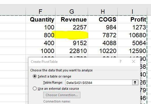
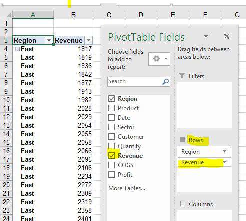
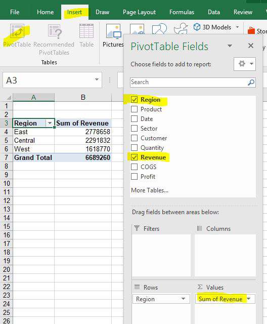
Now - even with an empty cell as shown in Figure 1, you can create the following pivot table in five mouse clicks:
- Insert
- Pivot Table
- OK
- Checkmark Region
- Checkmark Revenue
The feature has already made it to the Microsoft Insiders Channel. It has also made it to the Monthly (Targeted) Channel. It is definitely in version 1804, although it may have been in earlier versions. If your I.T. department has you set up for quarterly updates, watch for version 1804 to arrive and the problem will be solved.

Note that the new behavior is only for data where the column contains numbers or empty cells. If your column contains words like "None" or "N/A" or "Zero", you will continue to get a Count of Revenue instead of a sum. Also - beware the person who clears a cell by pressing the spacebar a few times. A cell that contains " " is not an empty cell. The best way to clear a cell is to select the cell and press the Delete key.
Watch Video
Title Photo: Maria Molinero on Unsplash