Excel 2020: Consolidate Quarterly Worksheets

April 16, 2020 - by Bill Jelen

Consolidate Quarterly Worksheets. Photo Credit: Pierre Châtel-Innocenti at Unsplash.com

There are two ancient consolidation tools in Excel.

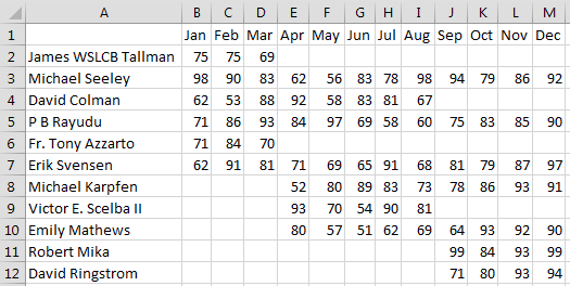
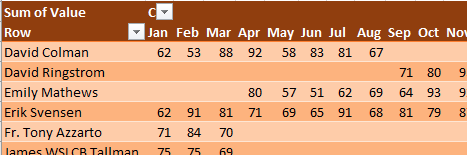
To understand them, say that you have three data sets. Each has names down the left side and months across the top. Notice that the names are different, and each data set has a different number of months.

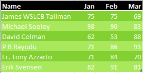
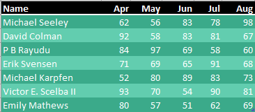
This is the first of three data sets to be consolidated. Names appear in A2:A7. Columns across the top are the months Jan, Feb, and Mar.

Data set 2 has five months instead of 3 across the top. Some people are missing and others are added.

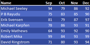
Some names in column A are the same as the previous image, but some are new. There are now five months across the top: Apr, May, Jun, Jul, and Aug.

Data set 3 has four months across the top and a few new names.

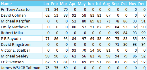
The final data set has months Sep, Oct, Nov, Dec. Again, names in column A. Some are repeated and some are new.

The Consolidate command will join data from all three worksheets in to one worksheet.

This is a cartoon illustrating what is about to happen. Three cartoon spreadsheets at the top are running towards each other, shouting "Let's Combine Into One Spreadsheet". At the bottom, a larger worksheet (with three faces and six arms) has all of the data from all three worksheets.

Illustration: Cartoon Bob D'Amico

You want to combine these into a single data set.

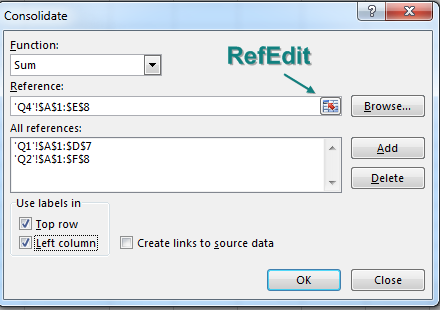
The first tool is the Consolidate command on the Data tab. Choose a blank section of the workbook before starting the command. Use the RefEdit button to point to each of your data sets and then click Add. In the lower left, choose Top Row and Left Column.

In the Consolidate dialog box, use the RefEdit button to point to the data on each of the three worksheets. In the lower left corner, make sure to choose Use Labels In: Top Row, Left Column.

This worksheet shows the result of the Consolidation. Names from all three lists appear in A2:A12. Across the top, all 12 months from Jan through Dec appear. Numbers populate the center of the grid. Several cells that should be numeric in the middle are empty instead of 0.

In the above figure, notice three annoyances: Cell A1 is always left blank, the data in A is not sorted, and if a person was missing from a data set, then cells are left empty instead of being filled with 0.

Filling in cell A1 is easy enough. Sorting by name involves using Flash Fill to get the last name in column N. Here is how to fill blank cells with 0:

Select all of the cells that should have numbers: B2:M11.
Press Ctrl+H to display Find & Replace.
Leave the Find What box empty, and type a zero in the Replace With: box.
Click Replace All.

The result: a nicely formatted summary report, as shown below.

Fill in the blanks with zero. Apply a table style.

The other ancient tool is the Multiple Consolidation Range pivot table. Follow these steps to use it:

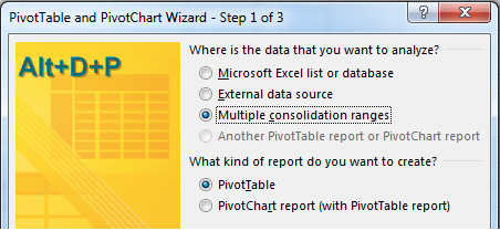
1. Press Alt+D, P to invoke the Excel 2003 Pivot Table and Pivot Chart Wizard.

2. Choose Multiple Consolidation Ranges in step 1 of the wizard. Click Next.

Press Alt+D P to open the legacy PivotTable and PivotChart Wizard. In Step 1 of 3, choose Multiple Consolidation Ranges.

3. Choose I Will Create the Page Fields in step 2a of the wizard. Click Next.

4. In Step 2b of the wizard, use the RefEdit button to point to each table. Click Add after each.

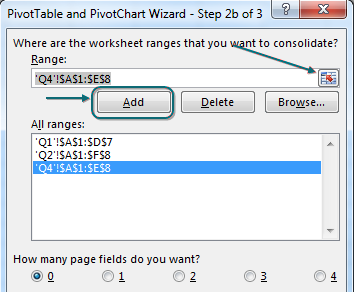
In the PivotTable wizard Step 2b of 3, specify all three ranges. Specify 0 page fields.

5. Click Finish to create the pivot table, as shown below.

The pivot table has names down the side and months across the top. It is very similar to the Consolidation report, but is refreshable.

Thanks to CTroy for suggesting this feature.

Title Photo: Pierre Châtel-Innocenti at Unsplash.com

This article is an excerpt from MrExcel 2020 - Seeing Excel Clearly.