Excel 2020: Create Your First Pivot Table

April 22, 2020 - by Bill Jelen

Create Your First Pivot Table. Photo Credit: Roman Bozhko at Unsplash.com

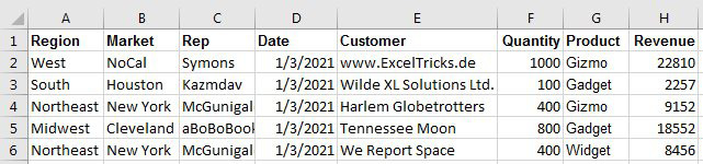
Pivot tables let you summarize tabular data to a one-page summary in a few clicks. Start with a data set that has headings in row 1. It should have no blank rows, blank columns, blank headings or merged cells.

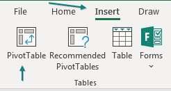
Columns are Region, Market, Rep, Date, Customer, Quantity, Product, and Revenue

Select a single cell in your data and choose Insert, Pivot Table.

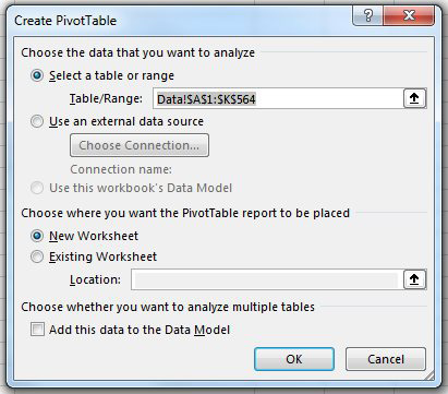
Detail of the Insert tab of the Ribbon. Pivot Table is the first icon on the Insert tab.

Excel will detect the edges of your data and offer to create the pivot table on a new worksheet. Click OK to accept the defaults.

The Create Pivot Table dialog identified the data as A1:K564 and offers to put the pivot table on a new worksheet.

Excel inserts a new blank worksheet to the left of the current worksheet. On the right side of the screen is the Pivot Table Fields pane. At the top, a list of your fields with checkboxes.

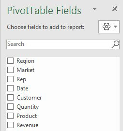
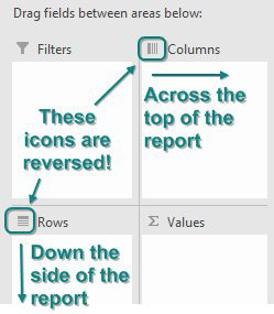
The top half of the Pivot Table Fields pane lists all of the fields from the original data set with a checkbox to the left of each one.

At the bottom are four drop zones with horrible names and confusing icons. Any fields that you drag to the Columns area will appear as headings across the top of your report. Any fields that you drag to the Rows area appear as headings along the left side of your report. Drag numeric fields to the Values area.

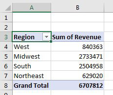
Four drop zones at the bottom of the Pivot Table Fields dialog are labeled Filters, Columns, Rows, and Values.

You can build some reports without dragging the fields. If you checkmark a text field, it will automatically appear in the Rows area. Checkmark a numeric field and it will appear in the Values area. By choosing Region and Revenue, you will create this pivot table:

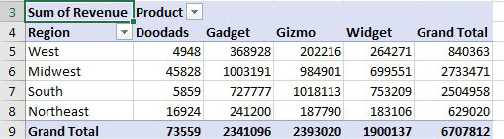
A pivot table with regions down column A and Sum of Revenue in column B. A Grand Total row appears below the data.

To get products across the top of the report, drag the Product field and drop it in the Columns area:

A pivot table with Products across the top and Region down the side.

Note

Your first pivot table might have the words "Column Labels" and "Row Labels" instead of headings like Product and Region. If so, choose Design, Report Layout, Show in Tabular Form. See Specify Defaults for All Future Pivot Tables.

Title Photo: Roman Bozhko at Unsplash.com

This article is an excerpt from MrExcel 2020 - Seeing Excel Clearly.