Excel 2020: Find the True Top Five in a Pivot Table

May 13, 2020 - by Bill Jelen

Excel Find the True Top Five in a Pivot Table. Photo Credit: Zhu Hongzhi at Unsplash.com

Pivot tables offer a Top 10 filter. It is cool. It is flexible. But I hate it, and I will tell you why.

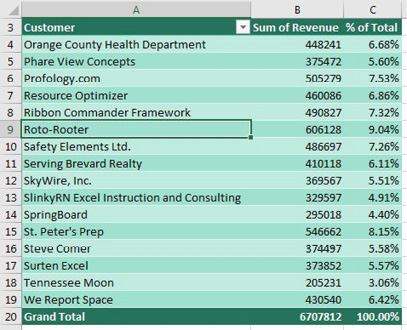
Here is a pivot table that shows revenue by customer. The revenue total is $6.7 million. Notice that the largest customer, Roto-Rooter, is 9% of the total revenue.

Customers in A4:A19 with a grand total in A20. The grand total is $6.7 Million. The largest customer is 606K and is 9.04% of the total.

What if my manager has the attention span of a goldfish and wants to see only the top five customers? To start, open the dropdown in A3 and select Value Filters, Top 10.

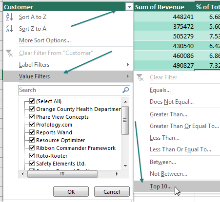
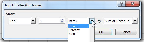
Open the Customers drop-down in cell A3. Choose Value Filters, Top 10. Note that other filters available are Greater Than, Less Than, Between, Not Between.

The super-flexible Top 10 Filter dialog allows Top/Bottom. It can do 10, 5, or any other number. You can ask for the top five items, top 80%, or enough customers to get to $5 million.

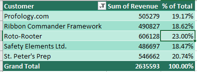
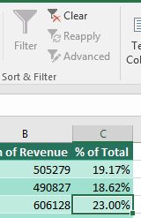
The Top 10 Filter dialog offers four controls. The first lets you choose Top or Bottom. The second is a spin button where you can enter a number. The third is a drop-down menu where you can choose Items, Percent, or Sum. The last is the field to use. In this screenshot, the settings are Top 5 Items by Sum of Revenue.

But here is the problem: The resulting report shows five customers and the total from those customers instead of the totals from everyone. Roto-Rooter, who was previously 9% of the total is 23% of the new total.

In this new pivot table with five customers, the Grand Total is now only $2.6 million (compared to $6.7 million before the filter). The largest customer accounts for 23% of the smaller grand total instead of 9% previously.

But First, a Few Important Words About AutoFilter

I realize this seems like an off-the-wall question. If you want to turn on the Filter dropdowns on a regular data set, how do you do it? Here are three really common ways:

Select one cell in your data and click the Filter icon on the Data tab or press Ctrl+Shift+L.
Select all of your data with Ctrl+* and click the Filter icon on the Data tab.
Press Ctrl+T to format the data as a table.

These are three really good ways. As long as you know any of them, there is absolutely no need to know another way. But here‘s an incredibly obscure but magical way to turn on the filter:

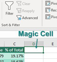
Go to your row of headers and then go to the rightmost heading cell. Move one cell to the right. For some unknown reason, when you are in this cell and click the Filter icon, Excel filters the data set to your left. I have no idea why this works. It really isn’t worth talking about because there are already three really good ways to turn on the Filter dropdowns. I call this cell the magic cell.

And Now, Back to Pivot Tables

There is a rule that says you cannot use AutoFilter when you are in a pivot table. See below? The Filter icon is grayed out because I’ve selected a cell in the pivot table.

With any cell in the pivot table selected, the Filter icon on the Data tab of the Ribbon is greyed out.

I don't know why Microsoft grays this out. It must be something internal that says AutoFilter and a pivot table can’t coexist. So, there is someone on the Excel team who is in charge of graying out the Filter icon. That person has never heard of the magic cell. Select a cell in the pivot table, and the Filter gets grayed out. Click outside the pivot table, and Filter is enabled again.

But wait. What about the magic cell I just told you about? If you click in the cell to the right of the last heading, Excel forgets to gray out the Filter icon!

Place the cell pointer in cell D3, which is the first blank cell to the right of the pivot table. The Filter icon should still be greyed out, but it is now available.

This is a cartoon illustration. An cartoon version of the AutoFilter is sneaking through a whole in the fence at Club Pivot Table. The sign on the fence says "No AutoFilter Allowed". — Illustration: George Berlin

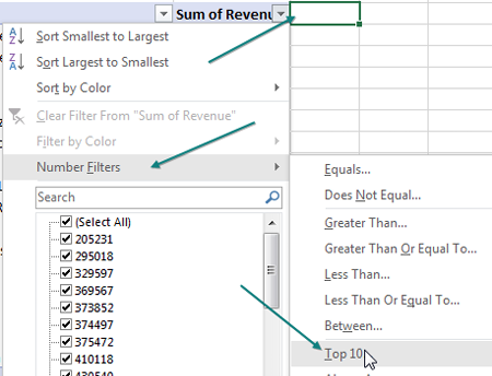
Sure enough, Excel adds AutoFilter dropdowns to the top row of your pivot table. And AutoFilter operates differently than a pivot table filter. Go to the Revenue dropdown and choose Number Filters, Top 10....

In contrast to the previous time you used Top 10, this time, you are opening a dropdown from the Sum of Revenue heading. Choose Number Filters, Top 10.

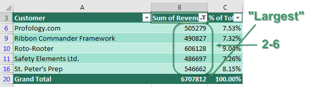
In the Top 10 AutoFilter dialog, choose Top 6 Items. That’s not a typo... if you want five customers, choose 6. If you want 10 customers, choose 11.

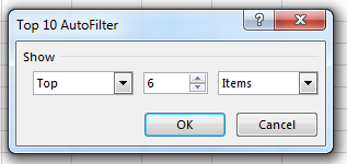
This dialog for Top 10 AutoFilter is narrower than before. Three controls offer Top, 6, Items.

To AutoFilter, the grand total row is the largest item in the data. The top five customers are occupying positions 2 through 6 in the data.

Success! Five customers and a Grand Total. The grand total is back to the "correct" $6.7 million and the largest customer is 9% of that Total.

Caution

Clearly, you are tearing a hole in the fabric of Excel with this trick. If you later change the underlying data and refresh your pivot table, Excel will not refresh the filter because, as far as Microsoft knows, there is no way to apply a filter to a pivot table!

Note

Our goal is to keep this a secret from Microsoft because it is a pretty cool feature. It has been “broken” for quite some time, so there are a lot of people who might be relying on it by now.

A Completely Legal Solution in Excel 2013+

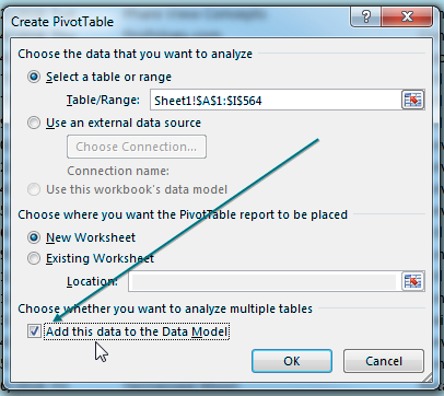
If you want a pivot table showing you the top five customers but the total from all customers, you have to move your data outside Excel. If you have Excel 2013 or newer running in Windows, there is a very convenient way to do this. To show you this, I’ve deleted the original pivot table. Choose Insert, Pivot Table. Before clicking OK, select the checkbox Add This Data To The Data Model.

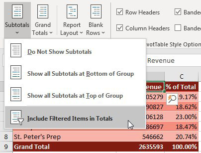
When creating the pivot table, choose the box for Add This Data To The Data Model. The box is in the lower left corner of the Create PivotTable dialog.

Build your pivot table as normal. Use the dropdown in A3 to select Value Filters, Top 10, and ask for the top five customers. With one cell in the pivot table selected, go to the Design tab in the Ribbon and open the Subtotals dropdown. The final choice in the dropdown is Include Filtered Items in Totals. Normally, this choice is grayed out. But because the data is stored in the Data Model instead of a normal pivot cache, this option is now available.

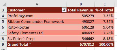
Because the pivot table is based on the Data Model, go to the Design tab, choose Subtotals and Include Filtered Items in Totals. This command is greyed out in regular pivot tables.

Choose the Include Filtered Items in Totals option, and your Grand Total now includes an asterisk and the total of all of the data, as shown below.

This pivot table shows the top five customers. The Grand Total row includes an asterisk and shows the total of all customers: $6.7 Million. The largest customer is correctly 9% of the Grand Total.

This magic cell trick originally came to me from Dan in my seminar in Philadelphia and was repeated 15 years later by a different Dan from my seminar in Cincinnati. Thanks to Miguel Caballero for suggesting this feature.

Title Photo: Zhu Hongzhi at Unsplash.com

This article is an excerpt from MrExcel 2020 - Seeing Excel Clearly.