
Excel 2020: Format as a Façade
November 25, 2020 - by Bill Jelen

Excel is amazing at storing one number and presenting another number. Choose any cell and select Currency format. Excel adds a dollar sign and a comma and presents the number, rounded to two decimal places. In the figure below, cell D2 actually contains 6.42452514. Thankfully, the built-in custom number format presents the results in an easy-to-read format.
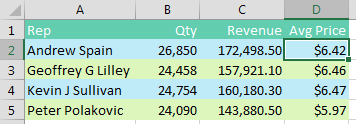
The custom number format code in D2 is $#,##0.00. In this code, 0s are required digits. Any #s are optional digits.
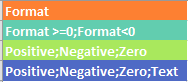
However, formatting codes can be far more complex. The code above has one format. That format is applied to every value in the cell. If you provide a code with two formats, the first format is for non-negative numbers, and the second format is for negative numbers. You separate the formats with semicolons. If you provide a code with three formats, the first is for positive, then negative, then zero. If you provide a code with four formats, they are used for positive, negative, zero, and text.
Even if you are using a built-in format, you can go to Format Cells, Number, Custom and see the code used to generate that format. The figure below shows the code for the accounting format.
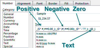
To build your own custom format, go to Format Cells, Number, Custom and enter the code in the Type box. Check out the example in the Sample box to make sure everything looks correct.
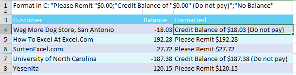
In the following example, three zones are used. Text in quotes is added to the number format to customize the message.
If you create a zone for zero but put nothing there, you will hide all zero values. The following code uses color codes for positive and negative. The code ends in a semicolon, creating a zone for zero values. But since the zone is empty, zero values are not shown.
![You can assign colors to positive and negative numbers. This number format is [Green]0;[Blue]-0; the final semicolon creates a zone for zero. By putting nothing there, you will hide the zero values.](/img/content/2020/11/XLFig381.png)

You can extend this by making all zones blank. A custom format code ;;; will hide values in the display and printout. However, you‘ll still be able to see the values in the formula bar. If you hide values by making the font white, the ;;; will stay hidden even if people change the fill color. The following figure includes some interesting formatting tricks.
![There are a lot of formatting tricks in this screenshot. A number format of **0.00 will fill everything to the left of the number with asterisks. *!0 will fill the blank space to the left of the number with exclamation points. A comma after the zero divides the number by 1000. So 0,K will display numbers in thousands. 0,,"M" will display numbers in millions. You can yell at people who enter text where a number should be: 0;-0;0;"Enter a number!". You can change the color based on conditions: [Red][<70]0;[Blue][>90]0;0. Another number formatting trick: an underscore followed by a character will leave enough white space to match the width of the character. This is supposed to be for getting numbers to line up when they have parentheses. But the screenshot uses 0_W_W0_N0_i0 to split 1234 up by varying amounts of white space.](/img/content/2020/11/XLFig383.png)
In B2 and B3, if you put ** before the number code, Excel will fill to the left of the number with asterisks, like the old check writer machines would do. But there is nothing that says you have to use asterisks. Whatever you put after the first asterisk is repeated to fill the space. Row 3 uses *! to repeat exclamation points.
In B4 and B5, each comma that you put after the final zero will divide the number by 1000. The code 0,K shows numbers in thousands, with a K afterward. If you want to show millions, use two commas. The "M" code must include quotation marks, since M already means months.
In B6, add a stern message in the fourth zone to alert anyone entering data that you want a number in the cell. If they accidentally enter text, the message will appear.
In B7 to B9, the normal zones Positives, Negatives, and Zero are overwritten by conditions that you put in square brackets. Numbers under 70 are red. Numbers over 90 are blue. Everything else is black.
In B10, those odd _( symbols in the accounting format are telling Excel to leave as much space as a left parenthesis would take. It turns out that an underscore followed by any character will leave as much white space as that character. In B10, the code contains 4 zeros. But there are different amounts of space between them. The space between the 1 and 2 is the width of 2 W characters. The space between 2 and 3 is the width of an N. The space between 3 and 4 is the width of a lowercase letter i.
The following figure shows various date formatting codes.
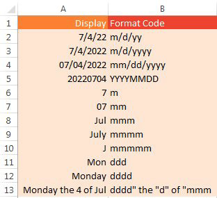
Note
The mmmmm format in row 8 is useful for producing J F M A M J J A S O N D chart labels.
Thanks to Dave Baylis, Brad Edgar, Mike Girvin, and @best_excel for suggesting this feature.
Title Photo: Unsplash.com
This article is an excerpt from MrExcel 2020 - Seeing Excel Clearly.