Excel 2020: Format One Cell in a Pivot Table

April 29, 2020 - by Bill Jelen

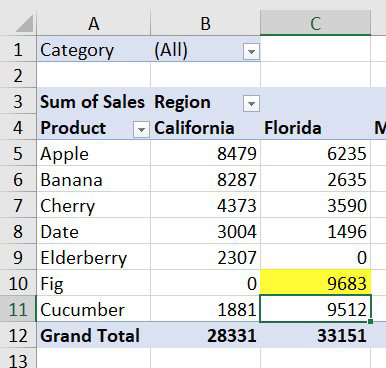
This is new in Office 365 starting in 2018. You can right-click any cell in a pivot table and choose Format Cell. Any formatting that you apply is tied to that data in the pivot table. In the figure below, Florida Figs have a yellow fill color.

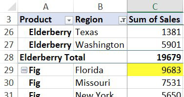
If you change the pivot table, the yellow formatting follows the Florida Fig.

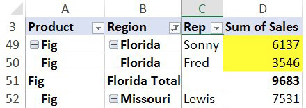
If you add a new inner field, then multiple cells for Florida Fig will have the fill color.

The formatting will persist if you remove Florida or Fig due to a filter. If you filter to vegetables, Fig is hidden. Filter to fruit and Fig will still be formatted. However, if you completely remove either Product or Region from the pivot table, the formatting will be lost.

Title Photo: Atilla Taskiran at Unsplash.com

This article is an excerpt from MrExcel 2020 - Seeing Excel Clearly.