
Excel 2020: Portable Formulas
June 24, 2020 - by Bill Jelen

If you have the full version of Power Pivot, you can use the DAX formula language to create new calculated fields. From the Power Pivot tab in the Ribbon, choose Measures, New Measure.
Give the field a name, such as Variance. When you go to type the formula, type =[. As soon as you type the square bracket, Excel gives you a list of fields to choose from.
Note that you can also assign a numeric format to these calculated fields. Wouldn’t it be great if regular pivot tables brought the numeric formatting from the underlying data?
![Defining a new calculated field or Measure. The formula is =[Sum of Revenue]-[Sum of Budget]. You can specify the formula is Currency with 0 decimal places.](/img/content/2020/06/XLFig251a.png)
In the next calculation, VariancePercent is reusing the Variance field that you just defined.
![The formula for VariancePercent is [Variance]/[Sum of Budget]. This one is formatted as a Number, Percentage, with 1 decimal place.](/img/content/2020/06/XLFig252.png)
So far, you've added several calculated fields to the pivot table, as shown below.
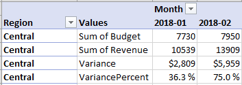
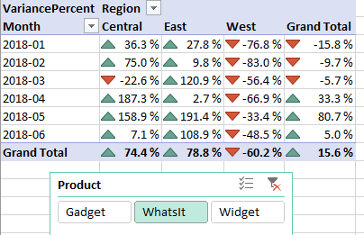
But you don’t have to leave any of those fields in the pivot table. If your manager only cares about the variance percentage, you can remove all of the other numeric fields.
Note that the DAX in this bonus tip is barely scratching the surface of what is possible. If you want to explore Power Pivot, you need to get a copy of Power Pivot and Power BI by Rob Collie.
Thanks to Rob Collie for teaching me this feature. Find Rob at PowerPivotPro.com.
Title Photo: Sheldon Nunes at Unsplash.com
This article is an excerpt from MrExcel 2020 - Seeing Excel Clearly.