Excel 2020: Slicers for Pivot Tables From Two Data Sets

June 29, 2020 - by Bill Jelen

Say that you have two different data sets. You want a pivot table from each data set and you want those two pivot tables to react to one slicer.

This really is the holy grail of Excel questions. Lots of Excel forums have many complicated ways to attempt to make this work. But the easiest way is loading all of the data into the workbook data model.

Both of the tables have to have one field in common. Make a third table with the unique list of values found in either column.

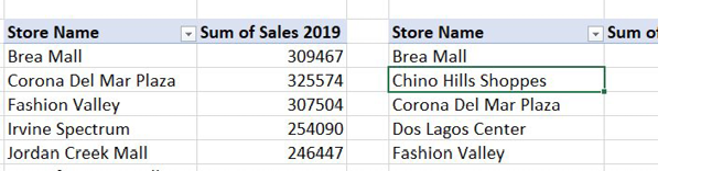
If the two tables are shown above, the third table has to have Store Names that are found in either table: Brea, Chino Hills, Corona Del Mar, Dos Lagos, Fashion Valley, Irvine, and so on.

Format all three of your tables using Ctrl+T.

Use the Relationships icon on the Data tab to set up a relationship from each of the two original tables to the third table.

If you have access to the Power Pivot grid, the diagram view would look like this:

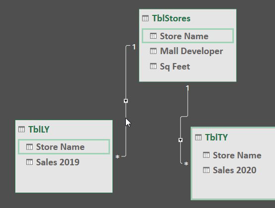
If not, the Relationships diagram should show two relationships, although certainly not as pretty as above.

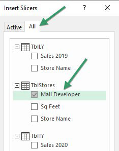
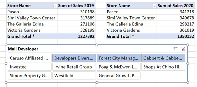
From either pivot table, choose Insert Slicer. Initially, that slicer will only show one table. Click on the All tab and choose Mall Developer from your third table.

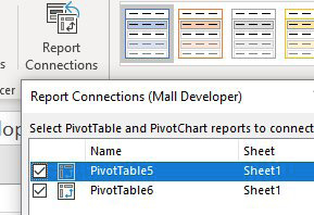
Try and choose a few items from the slicer. Watch your hopes get dashed as only one pivot table reacts. Once you recover, click on the Slicer. In the Slicer Tools Design tab of the Ribbon, choose Report Connections. Add the other pivot table to this slicer:

Finally, both pivot tables will react to the slicer.

Title Photo: Katie Smith at Unsplash.com

This article is an excerpt from MrExcel 2020 - Seeing Excel Clearly.