Excel 2020: Clean Data with Power Query

November 11, 2020 - by Bill Jelen

Clean Data with Power Query. Photo Credit: pan xiaozhen at Unsplash.com

Power Query is built in to Windows versions of Office 365, Excel 2016, Excel 2019 and is available as a free download in Windows versions of Excel 2010 and Excel 2013. The tool is designed to extract, transform, and load data into Excel from a variety of sources. The best part: Power Query remembers your steps and will play them back when you want to refresh the data. This means you can clean data on Day 1 in 80% of the normal time, and you can clean data on Days 2 through 400 by simply clicking Refresh.

I say this about a lot of new Excel features, but this really is the best feature to hit Excel in 20 years.

I tell a story in my live seminars about how Power Query was invented as a crutch for SQL Server Analysis Services customers who were forced to use Excel in order to access Power Pivot. But Power Query kept getting better, and every person using Excel should be taking the time to learn Power Query.

Get Power Query

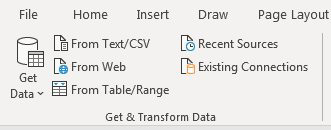
You may already have Power Query. It is in the Get & Transform group on the Data tab.

The Get & Transform Data group includes Get Data, From Text/CSV, From Web, From Table/Range, Recent Sources, Existing Connections.

But if you are in Excel 2010 or Excel 2013, go to the Internet and search for Download Power Query. Your Power Query commands will appear on a dedicated Power Query tab in the Ribbon.

Clean Data the First Time in Power Query

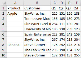
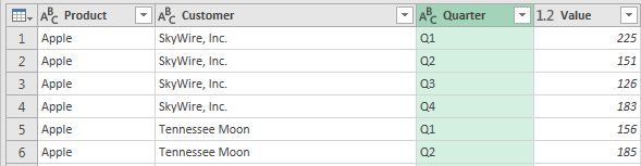
To give you an example of some of the awesomeness of Power Query, say that you get the file shown below every day. Column A is not filled in. Quarters are going across instead of down the page.

To start, save that workbook to your hard drive. Put it in a predictable place with a name that you will use for that file every day.

Products are in column A, but in an outline view where Applie appears in A2, followed by several blank cells. Banana is in A8 followed by more blank cells. Customers are in column B. Quarters are going across the worksheet in C, D, E, and F.

In Excel, select Get Data, From File, From Workbook.

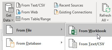
Browse to the workbook. In the Preview pane, click on Sheet1. Instead of clicking Load, click Edit. You now see the workbook in a slightly different grid—the Power Query grid.

Now you need to fix all the blank cells in column A. If you were to do this in the Excel user interface, the unwieldy command sequence is Home, Find & Select, Go To Special, Blanks, Equals, Up Arrow, Ctrl+Enter.

The blank cells in column A now say "null" in the Power Query Editor.

In Power Query, select Transform, Fill, Down.

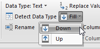
Choose column A. Open the Fill drop-down menu and choose FIll, Down.

All of the null values are replaced with the value from above. With Power Query, it takes three clicks instead of seven.

Next problem: The quarters are going across instead of down. In Excel, you can fix this with a Multiple Consolidation Range pivot table. This requires 12 steps and 23+ clicks.

In Power Query select the two columns that are not quarters. Open the Unpivot Columns dropdown on the Transform tab and choose Unpivot Other Columns, as shown below.

Select columns A and B in Power Query. On the Ribbon, choose Unpivot other columns.

Right-click on the newly created Attribute column and rename it Quarter instead of Attribute. Twenty-plus clicks in Excel becomes five clicks in Power Query.

You have four times as many rows. Columns A & B appear the same (except there are four rows for each previous one row). The Quarters that were going across columns C, D, E, and F now go down column C. The revenue from the data set is now in column D.

Now, to be fair, not every cleaning step is shorter in Power Query than in Excel. Removing a column still means right-clicking a column and choosing Remove Column. But to be honest, the story here is not about the time savings on Day 1.

But Wait: Power Query Remembers All of Your Steps

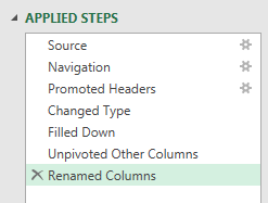
Look on the right side of the Power Query window. There is a list called Applied Steps. It is an instant audit trail of all of your steps. Click any gear icon to change your choices in that step and have the changes cascade through the future steps. Click on any step for a view of how the data looked before that step.

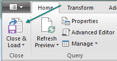
On the right side of the Power Query Editor, a list of Applied Steps. For this example, you have Source, Navigation, Promoted Headers, Changed Type, Filled Down, Unpivoted Other Columsn, Renamed Columns.

When you are done cleaning the data, click Close & Load as shown below.

Tip

If your data is more than 1,048,576 rows, you can use the Close & Load dropdown to load the data directly to the Power Pivot Data Model, which can accommodate 995 million rows if you have enough memory installed on the machine.

On the Home tab in Power Query, choose Close & Load.

In a few seconds, your transformed data appears in Excel. Awesome.

The transformed data is returned to a table in Excel.

The Payoff: Clean Data Tomorrow With One Click

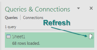
But again, the Power Query story is not about the time savings on Day 1. When you select the data returned by Power Query, a Queries & Connections panel appears on the right side of Excel, and on it is a Refresh button. (We need an Edit button here, but because there isn't one, you have to right-click the original query to view or make changes to the original query).

The Queries & Connections panel lists one query called Sheet1 with 68 rows loaded. If you make the panel wider and hover over Sheet1, a refresh icon appears.

It is fun to clean data on Day 1. I love doing something new. But when my manager sees the resulting report and says “Beautiful. Can you do this every day?” I quickly grow to hate the tedium of cleaning the same data set every day.

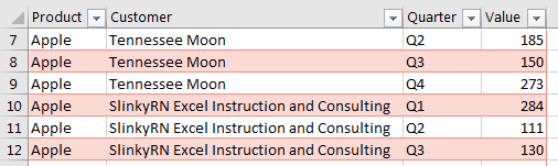
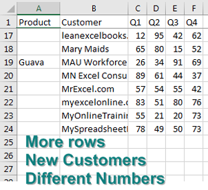
So, to demonstrate Day 400 of cleaning the data, I have completely changed the original file. New products, new customers, smaller numbers, more rows, as shown below. I save this new version of the file in the same path and with the same filename as the original file.

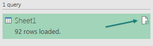
Change some data in the original worksheet. Add more rows. Type new customers. Change numbers.

If I open the query workbook and click Refresh, in a few seconds, Power Query reports 92 rows instead of 68 rows.

Click the Refresh icon in the Queries & Connections panel and it reports you have 92 rows loaded.

Cleaning the data on Day 2, Day 3, Day, 4,...Day 400,...Day Infinity now takes two clicks.

The new customers appear at the bottom of the table in Excel.

This one example only scratches the surface of Power Query. If you spend two hours with the book, M is for (Data) Monkey by Ken Puls and Miguel Escobar, you will learn about other features, such as these:

Combining all Excel or CSV files from a folder into a single Excel grid
Converting a cell with Apple;Banana;Cherry;Dill;Eggplant to five rows in Excel
Doing a VLOOKUP to a lookup workbook as you are bringing data into Power Query
Making a single query into a function that can be applied to every row in Excel

M is for Data Monkey - A guide to the M Language in Excel Power Query

For a complete description of Power Query, check out M Is for (Data) Monkey by Ken Puls and Miguel Escobar. By late 2019, the retitled second edition, Master Your Data, will be available.

Thanks to Miguel Escobar, Rob Garcia, Mike Girvin, Ray Hauser, and Colin Michael for nominating Power Query.

Title Photo: pan xiaozhen at Unsplash.com

This article is an excerpt from MrExcel 2020 - Seeing Excel Clearly.