
Excel 2024: Fast Worksheet Copy
February 26, 2024 - by Bill Jelen

Yes, you can right-click any sheet tab and choose Move or Copy to make a copy of a worksheet. But that is the very slow way to copy a worksheet. The fast way: Hold down the Ctrl key and drag the worksheet tab to the right.
The downside of this trick is that the new sheet is called January (2) instead of February but that is the case with the Move or Copy method as well. In either case, double-click the sheet name and type a new name.
Ctrl+drag February to the right to create a sheet for March. Rename February (2) to March.
Select January. Shift+select March to select all worksheets. Hold down Ctrl and drag January to the right to create three more worksheets. Rename the three new sheets.
Select January. Shift+select June. Ctrl+drag January to the right, and you've added the final six worksheets for the year. Rename those sheets.
Using this technique, you can quickly come up with 12 copies of the original worksheet quickly.

Illustration: Walter Moore
Bonus Tip: Put the Worksheet Name in a Cell
If you want each report to have the name of the worksheet as a title, use either of these
=TEXTAFTER(CELL("filename",A1),"]")
=TRIM(MID(CELL("filename",A1),FIND("]",CELL("filename",A1))+1,20)) &" Report"
The CELL() function in this case returns the full path\[File Name]SheetName. By looking for the closing square bracket, you can figure out where the sheet name occurs.
If you plan on using this formula frequently, set up a book.xltx as described at Use Default Settings for All Future Workbooks. In book.xltx, go to Formulas, Define Name. Use a name such as SheetName with a formula of =TEXTAFTER(CELL("filename",book.xltx!$A$1),"]"). Then, in any new workbook =SheetName&" Report" will work.
Bonus Tip: Add a Total Row and a Total Column with One AutoSum
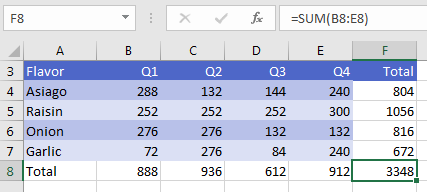
Say that you want to add a total row and a total column to a data set. Select all the numbers plus one extra row and one extra column. Click the AutoSum icon or press Alt+=.

Excel adds SUM functions to the total row and the total column as shown in the figure below.
Bonus Tip: Power Up the Status Bar Statistics
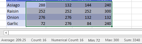
When you select two or more numeric cells, the total appears in the status bar in the lower right of the Excel window. When you see a total, right-click and choose Average, Count, Numerical Count, Minimum, Maximum, and Sum. You can now see the largest, smallest, and average just by selecting a range of cells.
Aha!
Aha!: Left-click any number in the status bar to copy that number to the clipboard.
Caution: Here is a fun fact: The numbers in the status bar are shown in the number format of the active cell. This is generally very useful and allows the status bar to show the Min and Max date as a date for example. But in one very confusing trick, someone had applied a crazy number format to hide the negative sign from a number to the top cell in a range. If you selected the range from the top, you had one number as the Sum in the status bar. If you selected from bottom to top, you had a different number in the status bar. It through a lot of really smart Excel people for a loop. For details, see Episode 2566 at the MrExcel YouTube channel.
Bonus Tip: Change All Sheets with Group Mode
|
Any time your manager asks you for something, he or she comes back 15 minutes later and asks for an odd twist that wasn't specified the first time. Now that you can create worksheet copies really quickly, there is more of a chance that you will have to make changes to all 12 sheets instead of just 1 sheet when your manager comes back with a new request. I will show you an amazingly powerful but incredibly dangerous tool called Group mode. |
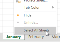 |
Say that you have 12 worksheets that are mostly identical. You need to add totals to all 12 worksheets. To enter Group mode, right-click on any worksheet tab and choose Select All Sheets.
The name of the workbook in the title bar now indicates that you are in Group mode.
![The title bar at the top of the Excel window shows the workbook name followed by the word Group enclosed in square brackets. [Group] is a very subtle indicator that the workbook is in group mode.](/img/content/2024/02/XLFig37.png)
Anything you do to the January worksheet will now happen to all the sheets in the workbook.
Why is this dangerous? If you get distracted and forget that you are in Group mode, you might start entering January data and overwriting data on the 11 other worksheets!
When you are done adding totals, don't forget to right-click a sheet tab and choose Ungroup Sheets.
Bonus Tip: Create a SUM That Spears Through All Worksheets
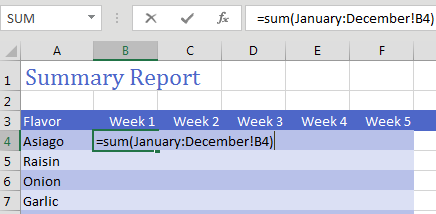
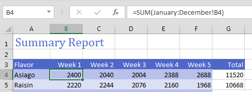
So far, you have a workbook with 12 worksheets, 1 for each month. All of the worksheets have the same number of rows and columns. You want a summary worksheet in order to total January through December.
To create it, use the formula =SUM(January:December!B4).
Copy the formula to all cells and you will have a summary of the other 12 worksheets.
Caution: I make sure to never put spaces in my worksheet names. If you do use spaces or punctuation, the formula would have to include apostrophes, like this: =SUM('Jan 2025:Mar 2025'!B4).
Tip
If you use 3D spearing formulas frequently, insert two new sheets, one called First and one called Last. Drag the sheet names so they create a sandwich with the desired sheets in the middle.Then, the formula is always =SUM(First:Last!B4).
Here is an easy way to build a 3D spearing formula without having to type the reference: On the summary sheet in cell B4, type =SUM(. Using the mouse, click on the January worksheet tab. Using the mouse, Shift+click on the December worksheet tab. Using the mouse, click on cell B4 on the December worksheet. Type the closing parenthesis and press Enter.
Bonus Tip: Use INDIRECT for a Different Summary Report
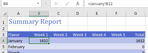
Say that you want to build the following report, with months going down column A. In each row, you want to pull the grand total data from each sheet. Each sheet has the same number of rows, so the total is always in row 12.
The first formula would be =January!B12. You could easily copy this formula to columns C:F, but there is not an easy way to copy the formula down to rows 5:15.
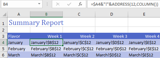
The INDIRECT function evaluates text that looks like a cell reference. INDIRECT returns the value at the address stored in the text. In the next figure, a combination of the ADDRESS and COLUMN functions returns a series of text values that tell Excel where to get the total.
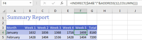
Wrap the previous formula in =INDIRECT() to have Excel pull the totals from each worksheet.
Caution: INDIRECT will not work for pulling data from other workbooks. Search the Internet for Harlan Grove PULL for a VBA method of doing this.
Thanks to Othneil Denis for the 3D formula tip, Olga Kryuchkova for the Group mode tip, and Al Momrik for status bar.
This article is an excerpt from MrExcel 2024 Igniting Excel
Title photo by Mathew Schwartz on Unsplash