
Excel 2024: Filter by Selection
February 17, 2024 - by Bill Jelen

The filter dropdowns have been in Excel for decades, but there are two faster ways to filter. Most people select a cell in the data, choose Data, Filter, open the dropdown menu on a column heading, uncheck Select All, and scroll through a long list of values, trying to find the desired item.
 |
One faster way is to click in the Search box and type enough characters to uniquely identify your selection. Once the only visible items are (Select All Search Results), Add Current Selection to Filter, and the one desired customer, press Enter. But the fastest way to Filter came from Microsoft Access. Microsoft Access invented a concept called Filter by Selection. It is simple: find a cell that contains the value you want and click Filter by Selection. The filter dropdowns are turned on, and the data is filtered to the selected value. Nothing could be simpler. Starting in Excel 2007, you can right-click the desired value in the worksheet grid, choose Filter, and then choose By Selected Cells Value. |
Guess what? The Filter by Selection trick is also built into Excel, but it is hidden and mislabeled.
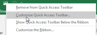
Here is how you can add this feature to your Quick Access Toolbar: Right-click anywhere on the Ribbon and choose Customize Quick Access Toolbar.
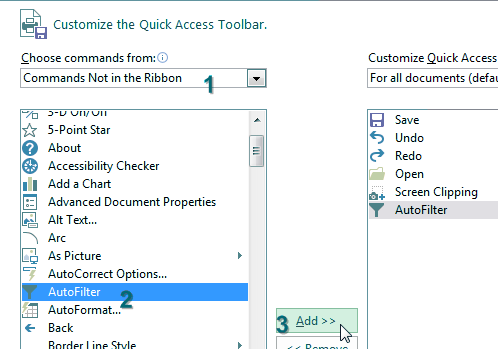
There are two large listboxes in the dialog. Above the left listbox, open the dropdown and change from Popular Commands to Commands Not In The Ribbon.
In the left listbox, scroll to the command AutoFilter and choose it.
In the center of the dialog, click the Add>> button. The AutoFilter icon moves to the right listbox, as shown below. Click OK to close the dialog.
That's right: The icon that does Filter by Selection is mislabeled AutoFilter.
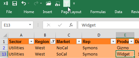
Here is how to use the command: Say that you want to see all West region sales of widgets. First, choose any cell in column B that contains West. Click the AutoFilter icon in the Quick Access Toolbar.
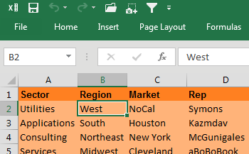
Excel turns on the filter dropdowns and automatically chooses only West from column B.
Next, choose any cell in column E that contains Widget. Click the AutoFilter icon again.
You could continue this process. For example, you could choose a Utilities cell in the Sector column and click AutoFilter.
Caution: It would be great if you could multi-select cells before clicking the AutoFilter icon, but this does not work. If you need to see sales of widgets and gadgets, you could use Filter by Selection to get widgets, but then you have to use the Filter dropdown to add gadgets. Also. Filter by Selection does not work if you are in a Ctrl+T table.
How can it be that this feature has been in Excel since Excel 2003, but Microsoft does not document it? It was never really an official feature. The story is that one of the developers added the feature for internal use. Back in Excel 2003, there was already an AutoFilter icon on the Standard toolbar, so no one would bother to add the apparently redundant AutoFilter icon.
This feature was added to Excel's right-click men, but three clicks deep: Right-click a value, choose Filter, then choose Filter by Selected Cell's Value.
Bonus Tip: Filter by Selection for Numbers Over/Under
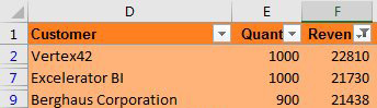
What if you wanted to see all revenue greater than $20,000? Go to the blank row immediately below your revenue column and type >19999. Select that cell and click the AutoFilter icon.
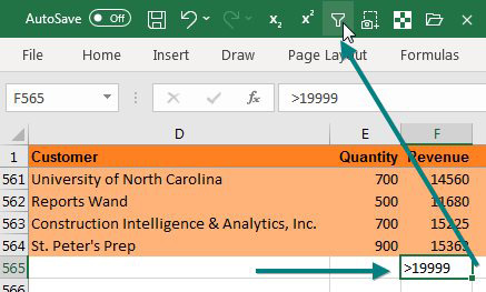
Excel will show only the rows of $20,000 or above.
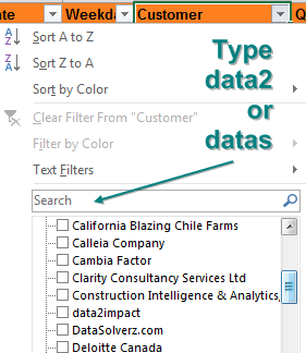
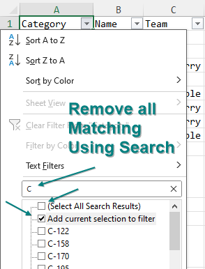
Bonus Tip: Remove Filter Items Using Search Box
|
What if you wanted to hide all items that contain certain text? Use the Filter Search box to find all matches. Unselect the box for Select All Search Results. This turns off all of the items that contain "C" in this case. Then, choose Add Current Selection to Filter. Apparently, since everything in the Current Selection is unchecked, you are adding the unchecked state to the current filter. It is a cool (but unintuitive) trick. Fold the corner of this page down, because it is a difficult trick to remember. |
 |
This article is an excerpt from MrExcel 2024 Igniting Excel
Title photo by Adi Goldstein on Unsplash