Excel 2020: Preview What Remove Duplicates Will Remove

August 26, 2020 - by Bill Jelen

Excel Preview What Remove Duplicates Will Remove. Photo Credit: Victor Garcia at Unsplash.com

The new Remove Duplicates tool added in Excel 2010 was a nice addition.

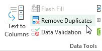
Remove Duplicates is found on the Data tab. It is to the right of the Text to Columns command and is often collapsed into a single column of 3 icons: Flash Fill, Remove Duplicates, and Data Validation.

However, the tool does remove the duplicates. Sometimes, you might want to see the duplicates before you remove them. And the Home, Conditional Formatting, Highlight Cells, Duplicate Values marks both instances of Andy instead of just the one that will be removed. The solution is to create a conditional formatting rule using a formula. Select A2:B14. Home, Conditional Formatting, New Rule, Use a Formula. The formula should be:

=COUNTIF($A$1:$A1,$A2)>0

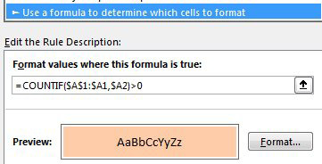
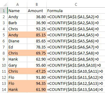
Use Conditional Formatting to highlight any duplicate values in orange.

It is hard to visualize why this will work. Notice that there is a dollar sign missing from $A$1:$A1. This creates an expanding range. In English the formula says "Look at all of the values from A1 to A just above the current cell and see if they are equal to the current cell". Only cells that return >0 will be formatted.

I've added the formula to column C below so you can see how the range expands. In Row 5, the COUNTIF checks how many times Andy appears in A1:A4. Since there is one match, the cell is formatted.

This screenshot shows the result. The first Andy in A2 is not orange. But the second Andy is A5 is orange. An extra set of formulas in column C shows how the range expands as the formula is copied down. While the first formula was =COUNTIF($A$1:$A1,$A2)>0, but the time it gets to the second Andy in row 5, the formula is =COUNTIF($A$1:$A5,$A5)>0.

Title Photo: Victor Garcia at Unsplash.com

This article is an excerpt from MrExcel 2020 - Seeing Excel Clearly.