
Excel 2020: Turn Data Sideways with a Formula
July 30, 2020 - by Bill Jelen

Someone built this lookup table sideways, stretching across C1:N2. I realize that I could use HLOOKUP instead of VLOOKUP, but I prefer to turn the data back to a vertical orientation.
Copy C1:N2. Right-click in A4 and choose the Transpose option under the Paste Options. Transpose is the fancy Excel word for “turn the data sideways.”
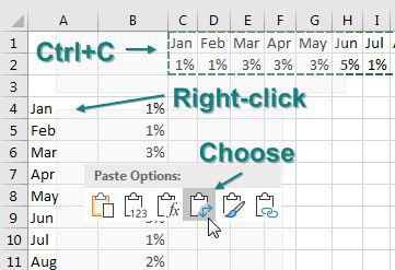
I transpose a lot. But I use Alt+E, S, E, Enter to transpose instead of the right-click.
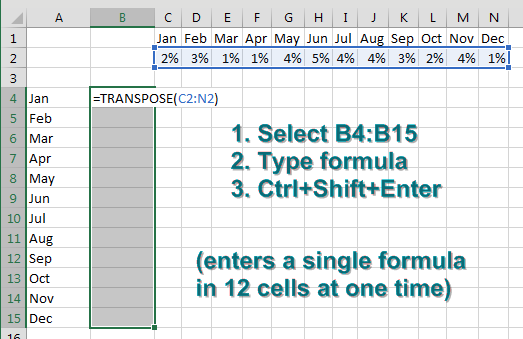
There is a problem, though. Transpose is a one-time snapshot of the data. What if you have formulas in the horizontal data? Is there a way to transpose with a formula?
The first way is a bit bizarre. If you are trying to transpose 12 horizontal cells, you need to select 12 vertical cells in a single selection. Start typing a formula such as =TRANSPOSE(C2:N2) in the active cell but do not press Enter. Instead, hold down Ctrl+Shift and then press Enter. This puts a single array formula in the selected cells. This TRANSPOSE formula is going to return 12 answers, and they will appear in the 12 selected cells, as shown below.
As the data in the horizontal table changes, the same values appear in your vertical table, as shown below.
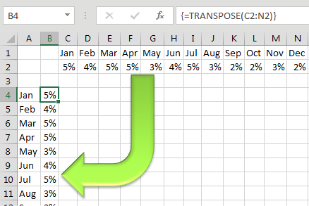
But array formulas are not well known. Some spreadsheet rookie might try to edit your formula and forget to press Ctrl+Shift+Enter.
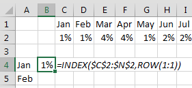
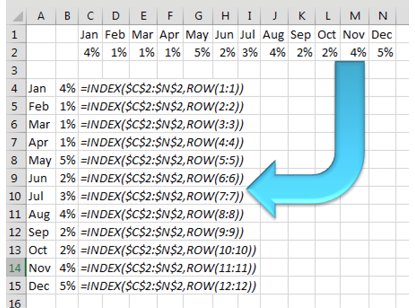
To avoid using the array formula, use a combination of INDEX and ROW, as shown in the figure below. =ROW(1:1) is a clever way of writing the number 1. As you copy this formula down, the row reference changes to 2:2 and returns a 2.
The INDEX function says you are getting the answers from C2:N2, and you want the nth item from the range.
In the figure below, =FORMULATEXT in column C shows how the formula changes when you copy down.
Title Photo: Pauline Loroy at Unsplash.com
This article is an excerpt from MrExcel 2020 - Seeing Excel Clearly.