Fast Excel Summary Reports with Pivot Tables

March 28, 2018 - by Bill Jelen

Microsoft says that 80% of people using Excel have never used a pivot table. As I near the end of my series of 40 Days of Excel, an introduction to pivot tables.

Pivot tables are miraculous. You are given a workbook with thousands of rows of detailed data. You can summarize that data in just a few clicks using a pivot table. I've written entire books on pivot tables, so today, I want to walk you through building your first pivot table.

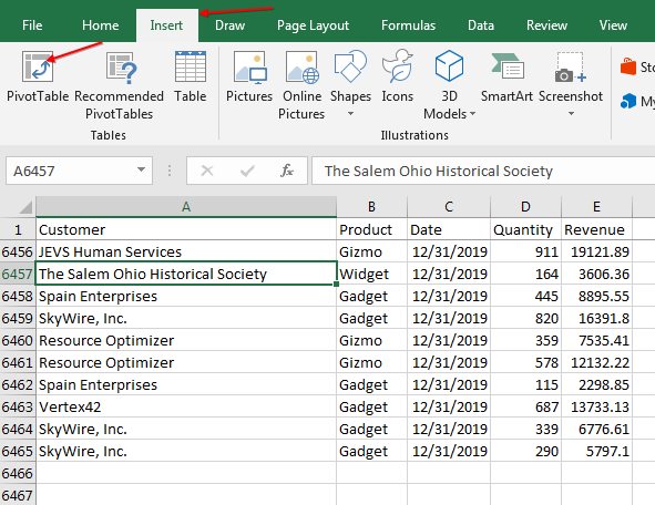
Say that you have 6464 rows of data with Customer, Product, Date, Quantity Revenue. You want to find the revenue for the top 5 customers who bought widgets.

1. Select one cell in your data set

2. On the Insert tab of the Ribbon, select Pivot Table

   

3. ---

   ---

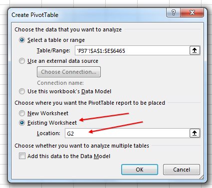
   In the Create PivotTable dialog, choose Existing Worksheet. Always leave a blank column between your data and the pivot table, so in this case, choose cell G2 for the place to hold your pivot table.

   

   The PivotTable Fields panel appears on the right side of your screen. At the top of the panel are a list of the fields in your data set. At the bottom are four drop zones with confusing names.

   

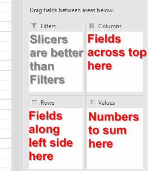
4. Drag the Customer field from the top of the PivotTable Fields list and drop it in the Rows drop zone.
5. Drag the Revenue field from the top of the PivotTable Fields list and drop it in the Values drop zone.
6. Drag the Product field to the Filters drop zone.

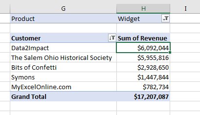
7. Open the filter drop-down in H2 and choose Widget. At this point, you will see a summary of the customers who bought widgets/

   

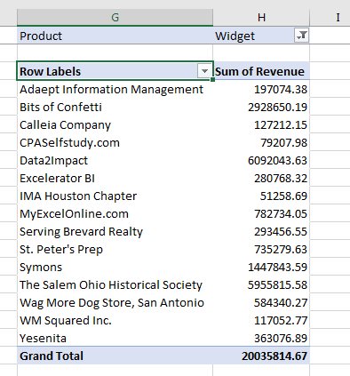
8. There are two PivotTable tabs in the Ribbon. Go to the Design tab. Choose Report Layout, Show in Tabular Form. This changes the heading in G3 from Row Labels to Customer. It also makes the pivot table better if you add more row fields later.
9. Open the drop-down in G3. Choose Value Filters, Top Ten. In the Top 10 Filter (Customer) dialog, choose Top, 5 Items by Sum of Revenue. Click OK.
10. Pivot tables never choose the right number format. Select all of the Revenue cells, from H4:H9. Assign a Currency format with 2 decimal places.
11. If you want the report sorted with the largest customer at the top, choose any one revenue cell and click the Sort Descending (ZA) icon on the Data tab. This is a shortcut for opening the drop-down in G3 and selecting Sort Z to A.

At this point, you've solved the original question:

However, Pivot Tables are easy to change. Now that you've answered the first question, try any of these:

• Change the dropdown in H1 from Widget to Gadget to see the top customers for gadgets.
• Double-click the revenue in H4 to see a list of all the records that make up that data. The report appears on a new worksheet to the left of the current worksheet.
• Click the Pivot Chart icon on the Analyze tab to chart the top 5 customers

These are just a few of the options in pivot tables.

I love to ask the Excel team for their favorite features. Each Wednesday, I will share one of their answers. Today's tip is from Excel Project Manager Ash Sharma.

Title Photo: Danist07 / Unsplash