Find the First Non-blank Value in a Row

January 20, 2021 - by Bill Jelen

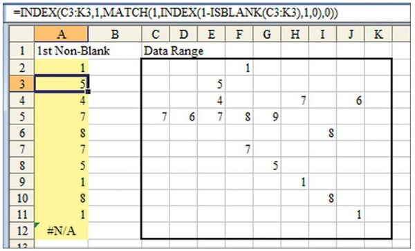
Challenge: You want to build a formula to return the first non-blank cell in a row. Perhaps columns B:K reflect data at various points in time. Due to the sampling methodology, certain items are checked infrequently.

Solution: In Figure 1, the formula in A4 is:

=INDEX(C4:K4, 1, MATCH(1, INDEX(1-ISBLANK(C4:K4), 1, 0), 0))

Although this formula deals with an array of cells, it ultimately returns a single value, so you do not need to use Ctrl+Shift+Enter when entering this formula.

Breaking It Down: Let’s start from the inside. The ISBLANK function returns TRUE when a cell is blank and FALSE when a cell is non-blank. Look at the row of data in C4:K4. The ISBLANK(C4:K4) portion of the formula will return:

{TRUE, TRUE, FALSE, TRUE, TRUE, FALSE, TRUE, FALSE, TRUE}

Notice that this array is subtracted from 1. When you try to use TRUE and FALSE values in a mathematical formula, a TRUE value is treated as a 1, and a FALSE value is treated as a 0. By specifying 1-ISBLANK (C4:K4), you can convert the array of TRUE/FALSE values to 1s and 0s. Each TRUE value in the ISBLANK function changes to a 0. Each FALSE value changes to a 1. Thus, the array becomes:

{0, 0, 1, 0, 0, 1, 0, 1, 0 }

The formula fragment 1-ISBLANK(C4:K4) specifies an array that is 1 row by 9 columns. However, you need Excel to expect an array, and it won’t expect an array based on this formula fragment. Usually, the INDEX function returns a single value, but if you specify 0 for the column parameter, the INDEX function returns an array of values. The fragment INDEX (1-ISBLANK (C4:K4),1,0) asks for row 1 of the previous result to be returned as an array. Here’s the result:

{0, 0, 1, 0, 0, 1, 0, 1, 0 }

The MATCH function looks for a certain value in a one-dimensional array and returns the relative position of the first found value. =MATCH (1, Array, 0) asks Excel to find the position number in the array that first contains a 1. The MATCH function is the piece of the formula that identifies which column contains the first non-blank cell. When you ask the MATCH function to find the first 1 in the array of 0s and 1s, it returns a 3 to indicate that the first non-blank cell in C4:K4 occurs in the third cell, or E4:

Formula fragment: MATCH(1, INDEX (1-ISBLANK (C4:K4), 1, 0), 0)

Sub-result: MATCH(1, {0, 0, 1, 0, 0, 1, 0, 1, 0}, 0)

Result: 3

At this point, you know that the third column of C4:K4 contains the first non-blank value. From here, it is a simple matter of using an INDEX function to return the value in that non-blank cell. =INDEX(Array, 1, 3) returns the value from row 1, column 3 of an array:

Formula fragment: =INDEX(C4:K4, 1, MATCH (1, INDEX (1-ISBLANK (C4:K4),1,0),0))

Sub-result: =INDEX(C4:K4, 1, 3)

Result: 4

Additional Details: If none of the cells are non-blank, the formula returns an #N/A error.

Alternate Strategy: Subtracting the ISBLANK result from 1 does a good job of converting TRUE/FALSE values to 0s and 1s. You could skip this step, but then you would have to look for FALSE as the first argument of the MATCH function:

=INDEX(C4:K4, 1, MATCH(FALSE, INDEX(ISBLANK(C4:K4), 1, 0), 0))

Summary: The formula to return the first non-blank cell in a row starts with a simple ISBLANK function. Using INDEX to coax the string of results into an array allows this portion of the formula to be used as the lookup array of the MATCH function.

Source: "1st occurance of non blank cell" on the MrExcel Message Board.

Title Photo: Ian Stauffer at Unsplash.com

This article is an excerpt from Excel Gurus Gone Wild.