How to Wrap Data to Multiple Columns in Excel

April 19, 2018 - by Bill Jelen

Gwynne has 15 thousand rows of data in three columns. She would like to have the data print with 6 columns per page. For example, the first 50 names in A2:C51, then the next 50 names in E2:G51. Then move the third 50 rows to A52:C101 and so on.

Rather than solve this with formulas, I am going to use a little Excel VBA to re-arrange the data.

The VBA macro will leave the data in A:C. A blank column will appear in D. The new data will appear in D:F, blank column in G, new data in H:J.

Note

Almost 10 years ago, I answered a question on how to snake 1 column in to 6 columns. In the case, the data was arranged horizontally, with Apple in C1, Banana in D1, Cherry in E1, ... Fig in H1, then Guava starting in C2 and so on. Back then, I answered the question using formulas. You can watch that old video : here.

The first step is to figure out how many rows fit on your printed page. Do not skip this step. Before you start with the macro, you need to do all of these things:

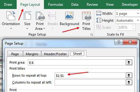
Set the margins on the Page Layout tab of the Ribbon
If you want your headings from Row 1 to repeat on each page, use Page Layout, Rows to Repeat at Top, and specify 1:1
Specify any headers and footers that will appear on each page.
Copy the headings from A1:C1 over to E1:G1.
Copy the headings from A1:C1 over to I1:K1.
Specify E:K as the print range
Fill the numbers 1 to 100 in E2:E101 with =ROW()-1

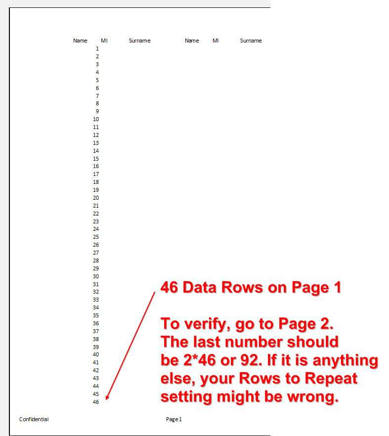
Setup the printed page. — Setup the page to be printed.

Once all of your page settings are correct, use Ctrl + P to display the Print Preview document. If necessary, click the Show Print Preview tile in the middle of the screen. In the Print Preview, find the last row number on page 1. In my case, it is 46. This will be an important number going forward.

To create the macro, follow these steps:

Save your workbook as a new name in case something goes wrong. For example: MyWorkbookTestCopy.xlsx
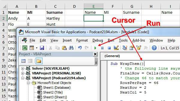
Press Alt + F11 to open the VBA Editor
From the VBA menu, choose Insert, Module

Copy the following code and paste to the code window

Sub WrapThem()
    ' the following line says XLUP not x1up !
    FinalRow = Cells(Rows.Count, 1).End(xlUp).Row
    ' Change 46 to match your Rows Per Page
    RowsPerPage = 46
    NextRow = 2
    NextCol = 5
    
    For i = 2 To FinalRow Step RowsPerPage
        Cells(NextRow, NextCol).Resize(RowsPerPage, 3).Value = _
            Cells(i, 1).Resize(RowsPerPage, 3).Value
        If NextCol = 5 Then
            NextCol = 9
        Else
            NextCol = 5
            NextRow = NextRow + RowsPerPage
        End If
    Next i
End Sub

Find the line that says RowsPerPage = 46 and replace the 46 with the number of rows that you found in your Print Preview.

Here are a few other things you might have to change depending on your data:

The FinalRow = line looks for the last entry in column 1. If your data started in column C instead of column A, you would change this:

FinalRow = Cells(Rows.Count, 1).End(xlUp).Row

to this

FinalRow = Cells(Rows.Count, 3).End(xlUp).Row

In this example, the first place for the new data will be cell E2. This is row 2, column 5. If you have five lines of titles and your new data is going to start in G6, you would change NextRow = 2 to NextRow = 6. Change NextCol = 5 to NextCol = 7 (because column G is the 7th column).

In this example, the data starts in A2 (right after headings in row 1). If you have 3 lines of headings, your data would start in A4. Change this line:

For i = 2 To FinalRow Step RowsPerPage

to this line:

For i = 4 To FinalRow Step RowsPerPage

My output columns appear in column E (5th column) and column I (9th column). Let's say you have four columns of data. The original data is in B:E. Put the first set of columns in G:J and L:O. G is the 7th column. L is the 12th column. In the following text, change 3 to 4 in two places because you have 4 columns instead of 3. Change 5 to 7 in two places because the first output column is G instead of E. Change 9 to 12 because the second output column is L instead of I.

Change this:

Cells(NextRow, NextCol).Resize(RowsPerPage, 3).Value = _
            Cells(i, 1).Resize(RowsPerPage, 3).Value
        If NextCol = 5 Then
            NextCol = 9
        Else
            NextCol = 5
            NextRow = NextRow + RowsPerPage
        End If

to this:

Cells(NextRow, NextCol).Resize(RowsPerPage, 4).Value = _
            Cells(i, 1).Resize(RowsPerPage, 4).Value
        If NextCol = 7 Then
            NextCol = 12
        Else
            NextCol = 7
            NextRow = NextRow + RowsPerPage
        End If

You are now ready to run the macro. Save the workbook one last time.

In the VBA window, click anywhere inside the macro. In the figure below, the cursor is right after Sub WrapThem(). Click the F5 key or click the Run icon as shown below.

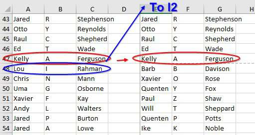
Switch back to Excel. You should see results like this:

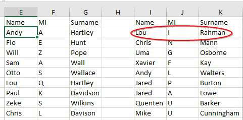
Make sure that the last name on page 1 column E is correctly followed by the first name in page 1 column I.

Watch Video

These steps are explained in this video:

Video Transcript

Learn Excel for MrExcel Podcast, Episode 2194: Wrapping Columns.

Hey, welcome back to MrExcel netcast, I'm Bill Jelen. Today's question, sent in by Gwen. Gwen is watching video 984, which was called Sneaking Columns. This is from years ago, and I actually used a formula to solve this back then, but this twins problem is more complicated.

So she has a three column worksheet with around 15,000 rows. and needs to make each page six columns. So, on the first page, these 60 cells; and then next to it, the next 60 cells. Now, Gwen has figured out that she can fit about 60 rows. But for anyone else watching this, the most important part here is to figure out how many rows because you'll really screw things up if you make any of these changes after the fact.

Alright, so for me, what I'm going to do is I'm going to come here to page layout, I'm gonna declare that these seven columns are going to be my print area-- Print Area, Set Print Area. I'm going to go into Print Titles and say that “Rows to repeat at top” is 1:1. I'm going to go... Actually, I'd like to use Margins here-- Margins, Narrow, and then back in the Page Setup, Header/Footer, and choose whatever my, you know, Custom Footer should be-- Confidential. Do all of the those settings, anything you're ever going to change first. Alright? Because that's going to change the number of rows per page.

Now, I'm going to type in the number 1 here, this is just going to be some temporary data. I'm going to hold down the Ctrl key and grab the Fill handle, and go down until I'm sure I'm past the first page like that. And then, we'll just do a Print Preview-- Ctrl+P, Show Print Preview-- and you'll notice that I have 46 rows that fit on the first page. And let's just check, go to the second page-- so 46 plus 46 is 92, so we're getting 46 rows per page, 46 rows per page. That number is incredibly important-- 46. In fact, I'm going to write it down over here just so I don't forget-- 46 rows per page.

Alright, now, I'm going to solve this today with a Macro; back in video 984, I used some complex formulas to do it, but today a macro feels better. If you've never used macros before don't be intimidated. Here's how we start: We press Alt+F11-- Alt+F11-- that brings open this screen and actually, the very first time that you open Alt+F11, it's going to be just a big gray screen-- probably a lot like this-- like that. So you want to say, View, Project Explorer, Find your workbook here, and say Insert Module-- I've already done that-- and what we'll get-- and what we get-- is a white screen. And over here in this white screen, you're going to type this code, alright? The word "Sub" which means that this is a subroutine, and then any naming you want-- I call it WrapThem, no spaces there, so just jam everything together-- open and closing parenthesis. Then we're we're going to create a variable: FinalRow = Cells(Rows.Count, 1).End, and these four letters here are XL, not X1-- everybody screws this up, XL. And you can type it in all caps if you want but they're going to change it back to that format where the L looks like a 1-- don't put a 1 there. Rows.Per.Page-- and this is where you put whatever number you figured out. Now, for me it's 46; for Gwen, it sounds like it's 60. And then, the next row where we want the first data to go is Row 2, and then the next column-- 1, 2, 3, 4, 5-- is Column 5.

Alright, so I set this up. And then, the rest of this is going to be very, very generic. it's going to work with, you know, any size data set: For I (it's a variable) = 2 To FinalRow (that's how many rows we had) Step (that means every time through the loop we're going to increase by) RowsPerPage (which in this case is 46, for Gwen's case it's going be 60). We're going to say: Cells(NextRow, NextCol) -- so, next row's going to be 2, Column 5-- .Resize(RowsPerPage, 3) -- resize 46 rows, 3 columns-- .Value = _ (and that's an underscore there) It's going to be equal to Cells(1, 1) -- so whatever is in Row 2 comma 1, Column 1-- .Resize(RowsPerPage, 3).Value. And then, what we have to do is, we have to be a little bit clever here about after we paste the first 46 times 46 rows, by 3 columns.

Where do we go next? There, right? So, if currently, the next column is pointing to Column E, well, then I need the next one to go to Column I. I is the ninth column. Alright. So that's why we say NextCol = 5. But if we're not... NextCol = 5 that means our NextCol = 9. Then we're going to reset the next group back to Column E and the NextRow is going to be = whatever the previous row was, + 46. And then next time.. now here, let's just walk through this, you don't have to run it one step at a time. But I'm going to do that with F8-- just to see what we get here.

And so, what we've learned, is the final row is real-- 15,582. We're about to write to row 2, column 5. And so: For I = 2 To FinalRow. The first time through, I is going to be equal to 2. We're going to say that Row 2, Column 5, is going to be equal to Row 2, Column 1-- 46 rows, 3 columns. I want to run this with F8. We'll look over here in the spreadsheet and we'll see that it turned out those first 46 came to this area. Alright. But, we're going to let this run again. Alright.

Now, the second time through the loop, the I has jumped up from 2 to 48. Alright. And so this time, we're going to be running to Row 2, Column 9, and we're going to be getting data from Row 48. Alright, now let's go check this one right here. So, what we see is Andy Hartley-- that works great-- down here at the end, Kelly Ferguson. But the next person should be Lue Rahman-- Rahman-- and that works, and it goes down to Lue Harvey, right there. Alright. Now, what we're hoping next time, is we get Barb Davison. I'll press F8 few more times, here's the next one and we look, and it's now writing to Row 48. Alright. And it's Barb Davison, and it appears to be working. At this point, I'm happy with it, I'm just going to click run.

And, actually, you don't have to go-- if you're not creating a video to explain this to somebody-- you don't have to go through and press F8; you could just come up here, click inside WrapThem, click run, and that fast it will take your data and wrap it into two columns.

Now, some things I see here-- Surname isn't wide enough, that should not affect our page layout, I'm hoping. And when I do Print Preview, I now have 170 pages. Data there, Page 2, Page 3, Page 4. Now, if we would change the margins at this point, everything is going to be screwed up-- it's going to be horrible. That's why it's really, really important, right up front, you have to do all of your page layout things before you calculate that 46. Now, of course, at this point, Save your workbook with a new name, alright? We don't want to destroy the personal workbook. And then you can delete columns A through D, and you have your results.

Now, if you want to learn about macros-- macros are incredibly powerful-- we probably could have solved this with a formula. And, certainly, the me from 10 years ago solved it with a formula, but at this point in my life, just a simple little 15 line macro is a lot easier. This book, by Tracy Syrstad and myself, will teach you all about macros.

Alright, wrap-up for this Episode: How to wrap 3 columns of data in 2 sets of columns per page. The super important step, you have to do all the page setup things first, Rows to Repeat at Top, Margins, Header/Footer, and then just type some numbers-- 1 through whatever-- I use the Fill handle with control; go to Print Preview, How many rows per page; switch over to Alt+F11; Insert a module and then type the code that I showed you in the video; click run. And most of the time, I advise people to save your workbook as xlsm, but in this case this was a one-time thing, I'm suspecting. So if you're, you know, just want to have that macro disappear, keep it as xlsx, save the file, it'll warn you that you're about to lose your macro. That's probably okay, because we've solved the problem well.

Hey, I want to thank Gwen for sending that question in, I want to thank you for stopping by. We'll see you next time for another netcast from MrExcel.

Title Photo: Edgar Castrejon on Unsplash