Pivot Ranks Don’t Match RANK()

January 24, 2023 - by Bill Jelen

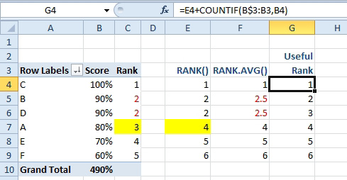
Problem: I set up a pivot table and showed the values as a rank, using Rank Largest to Smallest. Why is the fourth product assigned a rank of #3?

Excel has many ways of dealing with a tie when ranking. This example has six items and there is a two-way tie for second. In a pivot table rank, the ranks are 1, 2, 2, 3, 4, 5. Using the RANK() funtion the ranks are 1, 2, 2, 4, 5, 6. Using RANK.AVG, the ranks are 1, 2.5, 2.5, 4, 5, 6. The formula proposed in the book uses RANK+COUNTIF(B$3:B3,B4) and produces ranks 1, 2, 3, 4, 5, 6. — Figure 961. Why is C7 assigned a rank of 3?

Strategy: As if there is not enough controversy in the Excel ranking world, Excel came up with yet another way to handle ranking with pivot tables. The issue always centers around any ties and how the subsequent values are numbered.

Typically, if you have two values tied at #2, the next value would be assigned a rank of 4.

Starting in Excel 2010, the RANK.AVG would assign the tied values a 2.5, and assign the next item a rank of 4.

Pivot tables do something different, assigning both of the tie values a 2, then going to #3 for the next item.

If you need one of the methods shown in E:G, plan on adding a calculation next to your pivot table instead of using the built-in rank.

This article is an excerpt from Power Excel With MrExcel

Title photo by Tasha Lyn on Unsplash