Excel MVPs Attack the Data Cleansing Problem in Power Query

February 25, 2020 - by Bill Jelen

Note

This is one of a series of articles detailing solutions sent in for the Podcast 2316 challenge.

Excel MVP Oz Du Soleil from Excel on Fire channel on YouTube mentioned Brazilian Bull Rider Kaique Pachecho. Oz was the first person to notice that I went the slow way to add the four quarters.

Oz’s video is:
https://www.youtube.com/watch?v=OluZlF44PNI

His code is:

let
    Source = Excel.CurrentWorkbook(){[Name="UglyData"]}[Content],
    #"Removed Columns" = Table.RemoveColumns(Source,{"Column2", "Column3", "Column4", "Column5", "Column6"}),
    #"Transposed Table" = Table.Transpose(#"Removed Columns"),
    #"Promoted Headers" = Table.PromoteHeaders(#"Transposed Table", [PromoteAllScalars=true]),
    #"Changed Type" = Table.TransformColumnTypes(#"Promoted Headers",{{"Category Description", type text}, {"Administrative", type number}, {"Holiday", Int64.Type}, {"PTO/LOA/Jury Duty", Int64.Type}, {"Project A", type number}, {"Project B", type number}, {"Project C", type number}}),
    #"Added Conditional Column" = Table.AddColumn(#"Changed Type", "Custom", each if [Category Description] = "Q1" then null else if [Category Description] = "Q2" then null else if [Category Description] = "Q3" then null else if [Category Description] = "Q4" then null else [Category Description]),
    #"Filled Down" = Table.FillDown(#"Added Conditional Column",{"Custom"}),
    #"Renamed Columns" = Table.RenameColumns(#"Filled Down",{{"Custom", "Names"}}),
    #"Filtered Rows" = Table.SelectRows(#"Renamed Columns", each [Category Description] = "Q1" or [Category Description] = "Q2" or [Category Description] = "Q3" or [Category Description] = "Q4"),
    #"Reordered Columns" = Table.ReorderColumns(#"Filtered Rows",{"Names", "Category Description", "Administrative", "Holiday", "PTO/LOA/Jury Duty", "Project A", "Project B", "Project C"}),
    #"Unpivoted Other Columns" = Table.UnpivotOtherColumns(#"Reordered Columns", {"Names", "Category Description"}, "Attribute", "Value"),
    #"Pivoted Column" = Table.Pivot(#"Unpivoted Other Columns", List.Distinct(#"Unpivoted Other Columns"[#"Category Description"]), "Category Description", "Value", List.Sum),
    #"Inserted Sum" = Table.AddColumn(#"Pivoted Column", "Addition", each List.Sum({[Q1], [Q2], [Q3], [Q4]}), type number),
    #"Renamed Columns1" = Table.RenameColumns(#"Inserted Sum",{{"Addition", "TOTAL"}})
in
    #"Renamed Columns1"

Another solution, this one from Excel MVP John MacDougall.

John was the first to say that by deleting the two extra steps Power Query added, you eliminate the odd suffixes on the duplicate Q1 Q2 Q3 Q4 headings.
John used an Index column early that would be used at the end for sorting. But – John concatenated his index column after the category description. He used a vertical pipe character | so he could break the data out later.
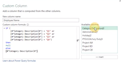
John typed his conditional column as a Custom column instead of using the Conditional Column interface.

Watch John’s video here:
https://www.youtube.com/watch?v=Dqmb6SEJDXI

Excel MVP Ken Puls, co-author of the M is for (Data) Monkey book sent in three solutions. His conditional column is probably the shortest.

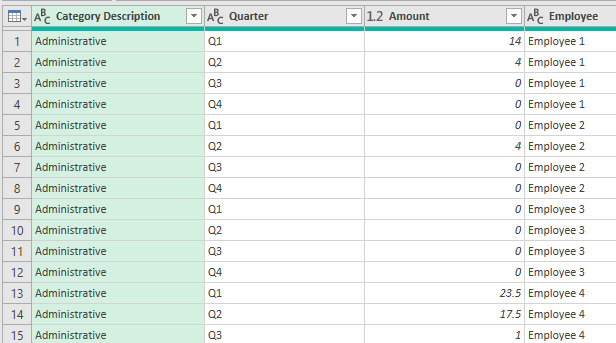
But Ken’s preferred solution ignores the original question. Instead of creating the table in Power Query, he creates a pivotable data set in Power Query and then finishes with a pivot table.

Ken’s final preview in Power Query looks like this:

Here is Ken’s code:

let
    Source = Excel.CurrentWorkbook(){[Name="UglyData"]}[Content],
    #"Promoted Headers" = Table.PromoteHeaders(Source, [PromoteAllScalars=true]),
    #"Changed Type" = Table.TransformColumnTypes(#"Promoted Headers",{{"Category Description", type text}, {"Dept. Total", type number}, {"Q1", type number}, {"Q2", type number}, {"Q3", type number}, {"Q4", Int64.Type}, {"Employee 1", type number}, {"Q1_1", type number}, {"Q2_2", type number}, {"Q3_3", Int64.Type}, {"Q4_4", Int64.Type}, {"Employee 2", Int64.Type}, {"Q1_5", Int64.Type}, {"Q2_6", Int64.Type}, {"Q3_7", Int64.Type}, {"Q4_8", Int64.Type}, {"Employee 3", Int64.Type}, {"Q1_9", Int64.Type}, {"Q2_10", Int64.Type}, {"Q3_11", Int64.Type}, {"Q4_12", Int64.Type}, {"Employee 4", type number}, {"Q1_13", type number}, {"Q2_14", type number}, {"Q3_15", type number}, {"Q4_16", Int64.Type}}),
    #"Removed Columns" = Table.RemoveColumns(#"Changed Type",{"Dept. Total", "Q1", "Q2", "Q3", "Q4"}),
    #"Unpivoted Other Columns" = Table.UnpivotOtherColumns(#"Removed Columns", {"Category Description"}, "Attribute", "Value"),
    #"Added Conditional Column" = Table.AddColumn(#"Unpivoted Other Columns", "Employee", each if Text.Contains([Attribute], "_") then null else [Attribute]),
    #"Filled Down" = Table.FillDown(#"Added Conditional Column",{"Employee"}),
    #"Split Column by Delimiter" = Table.SplitColumn(#"Filled Down", "Attribute", Splitter.SplitTextByEachDelimiter({"_"}, QuoteStyle.Csv, false), {"Attribute.1", "Attribute.2"}),
    #"Changed Type1" = Table.TransformColumnTypes(#"Split Column by Delimiter",{{"Attribute.1", type text}, {"Attribute.2", Int64.Type}}),
    #"Filtered Rows" = Table.SelectRows(#"Changed Type1", each ([Attribute.2] <> null)),
    #"Removed Columns1" = Table.RemoveColumns(#"Filtered Rows",{"Attribute.2"}),
    #"Renamed Columns" = Table.RenameColumns(#"Removed Columns1",{{"Attribute.1", "Quarter"}, {"Value", "Amount"}}),
    #"Changed Type2" = Table.TransformColumnTypes(#"Renamed Columns",{{"Category Description", type text}, {"Quarter", type text}, {"Amount", type number}, {"Employee", type text}})
in
    #"Changed Type2"

After creating this query as a connection only, he then uses a pivot table to create the final report.

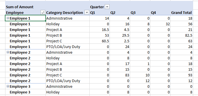
Solutions from other MVPs:

Wyn Hopkins code is here: Power Query: Dealing with Multiple Identical Headers.
Mike Girvin’s code is here: Power Query: Extracting Left 2 Characters From a Column.
Roger Govier’s formula solution is here: Formula Solutions.

Return to the main page for the Podcast 2316 challenge.

Read the next article in this series: Power Query: Beyond the User Interface: Table.Split and More.