
Replace 12 VLOOKUP with 1 MATCH
September 15, 2017 - by Bill Jelen

This is another formula speed example. Say that you have to do 12 columns of VLOOKUP. You can make it faster by using one MATCH and 12 INDEX functions.
In the following figure, you are going to have to do 12 VLOOKUP functions for each account number. VLOOKUP is powerful, but it takes a lot of time to do calculations.
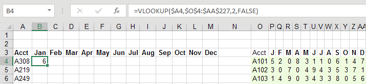
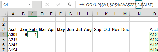
Plus, the formula has to be edited in each cell as you copy across. The third argument has to change from 2 to 3 for February, then 4 for March, and so on.
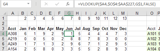
One workaround is to add a row with the column numbers. Then, the 3rd argument of VLOOKUP can point to this row. At least you can copy the same formula from B4 and paste to C4:M4 before copying the whole set down.
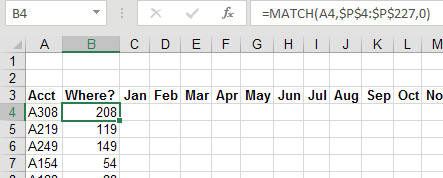
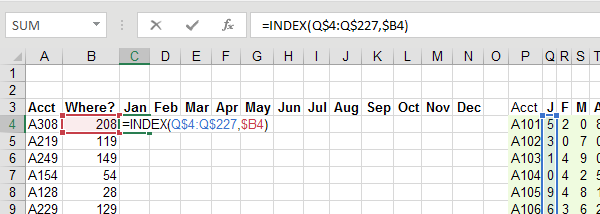
But here is a much faster approach. Add a new column B with Where? as the heading. Column B contains a MATCH function. This function is very similar to VLOOKUP: You are looking for the value in A4 in the column P4:P227. The 0 at the end is like the False at the end of VLOOKUP. It specifies that you want an exact match. Here is the big difference: MATCH returns where the value is found. The answer of 208 says that A308 is the 208th cell in the range P4:P227. From a recalc time perspective, MATCH and VLOOKUP are about equal.
I can hear what you are thinking. “What good is it to know where something is located? I’ve never had a manager call up and ask, ‘What row is that receivable in?’”
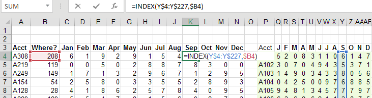
While humans rarely ask what row something is in, the INDEX function can use that position. The following formula tells Excel to return the 208th item from Q4:Q227.
As you copy this formula across, the array of values moves across the lookup table. For each row, you are doing one MATCH and 12 INDEX functions. The INDEX function is incredibly fast compared to VLOOKUP. The entire set of formulas will calculate 85% faster than 12 columns of VLOOKUP.
Watch Video
- Say that you have to do 12 columns of VLOOKUP
- Carefully use a single dollar sign before the column of the lookup value
- Carefully use four dollar signs for the lookup table
- You are still hard-coding the third column argument.
- One common solution is to add a row of helper cells with the column number.
- Another less-efficient solution is to use COLUMN(B2) inside the VLOOKUP formula.
- But, doing 12 VLOOKUP for each row is very inefficient
- Instead, add a helper column with a heading of WHERE and do a single Match.
- The MATCH takes as long as the VLOOKUP for January.
- You can then use 12 INDEX functions. These are incredibly fast compared to VLOOKUP.
- The INDEX will point to a single column of answers with $ before the rows.
- The INDEX will point to the helper column with a $ before the column.
Video Transcript
Learn Excel from MrExcel podcast, episode 2028 - Replacing Many VLOOKUPs with one MATCH!
Click that “i” on the top-right hand corner to get to the playlist, I'll be podcasting this entire book!
Hey, welcome back to the MrExcel netcast, I'm Bill Jelen! Well it's a classic problem, we have to do VLOOKUP once for every month, right? And you can be incredibly careful here about pressing F4 3 times to lock that down to the column, and then pressing F4 once the lock down the whole row. But when you get to this point, the ,2,FALSE that 2 is hard-coded, and as you copy that across, you're going to have to edit the 2 to a 3, right? Now, one inefficient way to do this, a way that I don't like is to use the column of B1. Column B1 is of course 2, but as you copy that across, see that it'll change to the column C1, which is 3, but think about this, this is constantly figuring out the column number over and over again. So what I see people do and why, you know, prefer more than the columns, is we'll Ctrl-drag that, put the numbers 2-13 up there in a helper cell, and then, when we get to this point, we go up and specify that column number. Press F4 2 times to lock it down to the row, ,FALSE and so on. But even with that method, VLOOKUP is incredibly inefficient, because it has to go search through all of these items here until it finds A308 and that's the figure out B4. When it then moves over to C4, it forgets that it just went and looked, and it starts all over again, alright. So you have one of the slowest functions in all of Excel, the VLOOKUP ,FALSE being done over and over and over for the same item.
So here's the much, much faster way to go, we're going to insert a helper column, and this helper column I call it Where? As in where the heck is A308? We'll use a =MATCH, look for A308 in the first row of the table, press F4 there, ,0 for an exact match, alright, it tells us that “Hey, look at that, it's in row, 6, how awesome is that?” But as we copy down, see, it's in different places all the time. Alright, now this match takes as long as the January VLOOKUP takes, there they're dead even, but here's the amazing thing. From there we never have to do a VLOOKUP for the rest of the row, we could just do =INDEX, INDEX says “Here's an array of answers.” I'm going to go to the January cells, and I'm going to very carefully here press F4 2 times so I lock it down to 4:227, but the Q is allowed to change as I move. Comma, and then it wants to know what row, well that's going to be the answer in B4, I'll press F4 3 times to get the $ before the B, alright, copy that across.
This formula, these INDEX formulas, these 12 will happen in less than the time it would take to do the February VLOOKUP, alright. If we put Charles Williams timer on this, this whole thing will calculate an about 14% of the time of 12 VLOOKUPs. Your manager doesn't want to see the Where? Fine, just hide that column, everything keeps working, alright, this is a beautiful way to speed up the 12 months or the 52 weeks of VLOOKUPs. Alright, this tip, and so many more tips, are in this book. Click the “i” on the top-right hand corner there, you can buy the book, $10 e-book, $25 for the print book, alright.
So today we had a problem where 12 columns of VLOOKUP, you can carefully put the $ in, but then that 3rd argument still has to be hardcoded. You could use column(B2), I'm not a fan of that, because there's hundreds of rows *12 columns where's calculating that over and over. Just use a helper cell in a row, put the numbers 2-12 and point to that, it's still inefficient, though, because VLOOKUP after it figures out January, it has to start back in the beginning for February. So I recommend adding a column with a heading of “Where?” and doing a single MATCH there. That MATCH takes as long as the VLOOKUP for January, but then the 12 INDEX functions will take less time than the VLOOKUP for February, and you've trimmed a whole bunch of time. Again, careful with the $ in the INDEX function in both places, one just before the rows, and the other one before the columns, a mixed reference in both of them.
Hey, I want to thank you for stopping by, we'll see you next time for another netcast from MrExcel!
Download File
Download the sample file here: Podcast2028.xlsx
Title Photo: roegger / Pixabay