
Replicate Pivot Table For Each Rep
August 16, 2017 - by Bill Jelen

There is an easy way to replicate a pivot table for each rep, product, whatever.
Here is a great trick that I learned from my coauthor Szilvia Juhasz.
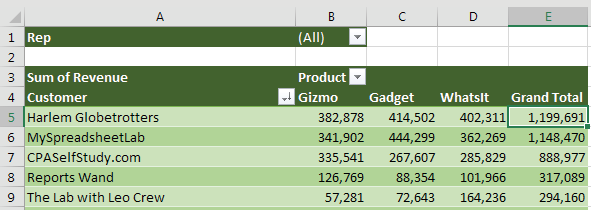
The pivot table below shows products across the top and customers down the side. The pivot table is sorted so the largest customers are at the top. The Sales Rep field is in the Report Filter.
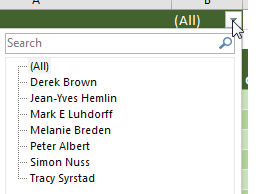
If you open the Rep filter dropdown, you can filter the data to any one sales rep.
This is a great way to create a report for each sales rep. Each report summarizes the revenue from a particular salesperson's customers, with the biggest customers at the top. And you get to see the split between the various products.
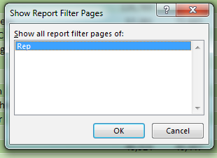
The Excel team has hidden a feature called Show Report Filter Pages. Select any pivot table that has a Report Filter. Go to the Analyze tab (or the Options tab in Excel 2007/2010). On the far left side is the large Options button. Next to the large Options button is a tiny dropdown arrow. Click this dropdown and choose Show Report Filter Pages.
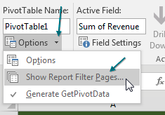
Excel asks which field you want to use. Select the one you want (in this case the only one available) and click OK.
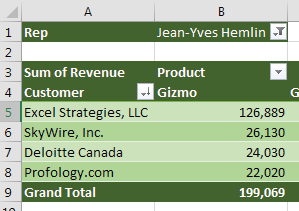
Over the next few seconds, Excel starts inserting new worksheets, one for each sales rep. Each sheet tab is named after the sales rep. Inside each worksheet, Excel replicates the pivot table but changes the name in the Report Filter to this sales rep.
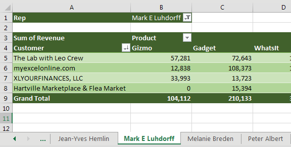
You end up with a report for each sales rep.
This would work with any field. If you want a report for each customer, product, vendor, or so on, add it to the Report Filter and use Show Report Filter Pages.
Thanks to Szilvia Juhasz for showing me this feature during a seminar I was teaching at the University of Akron many years ago. For the record, Szilvia was in row 1.
Watch Video
- There is an easy way to replicate a pivot table for each rep, product, whatever
- Create the pivot table
- To replace the Row Labels heading with a real heading, use Show in Tabular Form
- To replace Sum of Revenue, type a space and then Revenue
- Provided you select all value cells and the grand total, you can change the number format without going to Field Settings
- Greenbar effect using Design, Banded Rows, and then choosing from the Format gallery
- Add the "for each" field to the Filter area
- Go to the first Pivot table tab in the ribbon (Options in 2007 or 2010, Analyze in 2013 or 2016)
- Open the tiny dropdown next to Options
- Choose Show Report Filter Pages
- Confirm which field to use and click OK
- Excel will insert a new worksheet for each rep
- Thanks to L.A. Excel consultant Szilvia Juhasz for this trick
Video Transcript
Learn Excel for MrExcel Podcast, Episode 2005 -- Replicate Pivot Table For Each Rep
I'll be podcasting this entire book. Go ahead and subscribe to the MrExcel XL playlist up there in the top right-hand corner.
Alright, today's tip, is from my co-author Sylvia Juhasz. Sylvia came to one of my seminars at the University of Akron. Oh wow! 10, 12 years ago and she had a copy of my book: Pivot Table Data Crunching and she says why didn't you show this feature? And I said because as far as I know the feature doesn't work, but it did work.
Alright so here's what we're going to do. We're going to create a Pivot Table from this data. Insert Pivot Table. Okay, on a new worksheet, we're going to maybe show customers down the left-hand side and revenue; and then we want to create this report for either a product line manager, or for a sales rep. So we add those items to the filter.
Alright now, I would like to do a few things to customize this. First off, instead of the word row labels, I want to have the word Customer up there. So that's Report Layout, Show In Tabular Form. Instead of Sum of Revenue, I want to put space Revenue. Why don't I just put Revenue? Because they won't let you put Revenue, you have to put space either before or after, because revenue is already a name in the Pivot Table. Alright, so it's kind of a weird thing. We will format this as currency with zero decimal places, so it looks good. Maybe even come here on the Design Tab choose, Banded Rows and then some nice color. Maybe go with this green, because its revenue after all, right?
And then what we could do is if we wanted to see this report for just one product, or just one rep, we could open this Drop Down and see that, but I want to see it for all of the reps. I want to take this Pivot Table and replicate it for every single rep. Now they've really hidden this. Now go to the Analyze Tab. I see this options button? That's not what I want you to do. I want you to click the tiny little Drop Down and say Show Report Filter Pages and because I have two different things in the Report Filter Area: Sales Reps and Products. They offer me both. I'm going to choose rep and when I click OK, alright, they just took my Pivot Table and replicated it for every single item in the rep drop-down and on each one they chose that rep. Alright now obviously make sure your Pivot Table is formatted correctly before you go and create a whole bunch of different Pivot Tables, but this is a beautiful, beautiful trick.
And it's just one of the many tricks in this book. You can get the complete cross-referenced, all the podcast from August in September. 25 bucks in print or ten bucks as an e-book.
Alright, episode recap there is an easy way to replicate a Pivot Table for each rep, product or whatever. First create the Pivot Table and then whatever the “for each” field is: Sales, Rep or Product Line, add that to the Filter Area in the Pivot Table Tools Tab. Go to either Options in 2007 or 2010 or Analyze. It's the first tab and, in any case. There's a tiny Drop Down, next to Options. Open that, Choose Show Report Filter Pages, confirm which field to use, click OK and then Excel will jump into action and replicate that Pivot Table for each, whatever item it is that's in that field and I got this from LA based Excel consultant and trainer Sylvia Juhasz. If you're out in Southern California need Excel training or Excel work done, contact Sylvia Juhasz. She will do a great, great job for you.
Hey, I want to thank you for stopping by. We'll see you next time, for another netcast, from MrExcel.
Download File
Download the sample file here: Podcast2005.xlsx
Title Photo: klimkin / pixabay