
Round To Quarter Hour
May 29, 2018 - by Bill Jelen

Another question from my Atlanta Power Excel seminar:
How can you round billable time up to the next quarter hour?
Say that you keep a log of your billable time. You have a start time and an end time. A formula such as =E2-D2 will calculate the elapsed time.
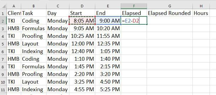
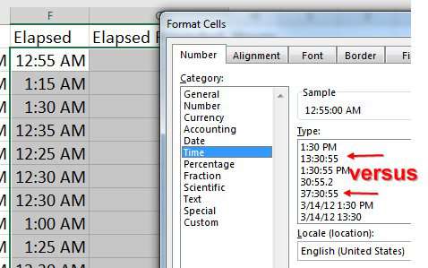
The result in F2 is 55 minutes. But the default formatting shows 12:55 AM. Choose the whole column. Press Ctrl + 1 to Format Cells. Select the Time category. Which of these should you use? For now, choose 13:30:55, but you will see later the problem with this selection.
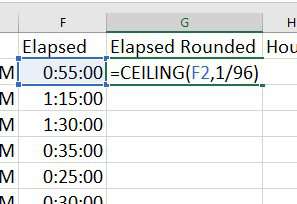
Your company policy is to round all billings up to the next quarter hour. Do this calculation: There are 24 hours in a day. There are 4 quarter hours in an hour. Multiply 24*4 to get 96. That means that a quarter hour is equivalent to 1/96 of a day.
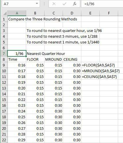
Use the formula =CEILING(F2,1/96) to round the elapsed time in F up to the next quarter hour. In Excel's method of storing time, Noon is 0.5. 6AM is 0.25. 12:15 AM is 1/96 or 0.010417. It is easier to remember 1/96 than 0.010417.
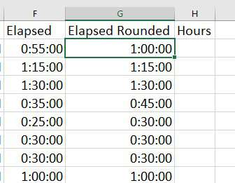
The results are shown below. Notice how the 35 minutes rounds up to 45 minutes. This seems to be the formula my attorney uses... haha, that's just a joke Esquire Dewey! Don't sue me! I know they use =CEILING(F2,4)...
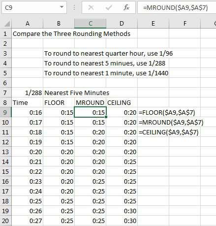
Pausing here... this article is rounding up to the next quarter hour because that is the method Larry in my seminar is using. There is a good chance that you company rounds to something else. The image below shows how to round to five minutes or 1 minute. You could use similar logic to round to the nearest 6 minutes (1/240) or 12 minutes (1/120).
Also - a gentle suggestion showing the difference between FLOOR, MROUND, and CEILING. The FLOOR function in B9:B22 always rounds down. The MROUND in C9:C22 rounds to the nearest. The CEILING in D9:D22 rounds up.
Note
The Excel tooltip will suggest that you use FLOOR.MATH or CEILING.MATH instead of FLOOR or CEILING. The new ".Math" versions of these functions handle negative numbers differently. Because time in Excel can never be negative, it is fine to use the regular FLOOR or CEILING.
Change the fraction from 1/96 to 1/288 to round to five minute increments.
Converting Times to Hours
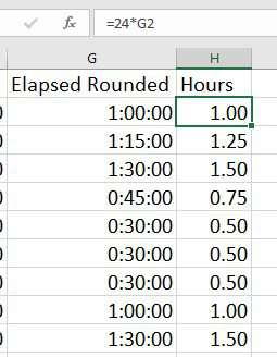
Another suggestion from Larry: Convert the times to real hours. That way, when you multiply by the billing rate per hour, the math will work. Take the rounded elapsed time and multiply by 24 to get a decimal number of hours. Make sure to format the result as a number with two decimal places and not a time.
Which Time Format to Use?
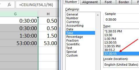
It is time to talk about those time formatting choices: You could have chosen 13:30, 13:30:55, or 37:30:55. In the screenshots above, I've used 13:30:55. The problem with this appears at the end of the week. When you total the decimal hours in column H, you have 53 billable hours. When you total the times in G, you get five hours. What is going on?
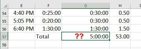
Both are correct, if you understand the number format that you selected. Say that you enter =NOW() in a cell. You could format the cell to show date & time, just date, or just time. Excel has no problem leaving off the May 29 portion of May 29 08:15:34 AM if you tell it to do that. The answer in cell G57 is "2 days and five hours". But when you chose 13:37:55 as the time format, you were telling Excel to leave off the number of days and only show you the hours, minutes, and seconds.
If you convert column G to use 37:30:55 format, then you get the correct number of hours:
The caption above that image captures the small problem with 37:30:55 format: it is showing seconds, which seems unneccesary since we are rounding to the nearest fifteen minutes. After choosing 37:30:55, click on the Custom category. You can see the number formatting code of [h]:mm:ss;@ is used. The square brackets around the H is the important part.
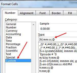
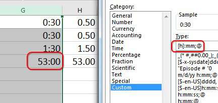
To show your times in hours and minutes, edit the number format to remove the :ss.
Watch Video
Today's video contains a bonus tip at the end for formatting decimals as a fraction.
Video Transcript
Learn Excel From MrExcel Podcast, Episode 2210: Round Up to the Next Quarter Hour.
Hey, welcome back to MrExcel netcast, I'm Bill Jelen. Today, another question from my Atlanta Power Excel seminar. Someone was doing a billing spreadsheet, and they wanted to round up to the next quarter hour, right? So, for each task here, they have a Client, Start Time, and End Time, and to calculate the Elapsed Time-- that's simple, if those are real times, or if they're just =E2-D2. So, that's saying 55 minutes, but it's saying it in a really weird way-- "12:55 AM." We want to go ahead and format this. Choose Time, and hey, look, there's a few different choices here: 13:30; 13:30:55, which would show the seconds; and then 37:30:55. Now, for right now, I'm going to choose the 13:30, but we're going to circle back later on and re-examine that choice. So, I choose OK and double-click to copy it down, and you see that it is just doing the math -- so here, 25 minutes. But, the person who asked this question-- the firm they work for-- they want to round up to the next quarter hour.
Alright, so, quarter hour. Let's think about times in Excel. Noon is 0.5. If I format that as a time-- 12:00:00 PM. And if I do 0.25, that'll be 6:00:00 AM. Alright, so the way this works is that one full day is the number 1.0, and so, if we wanted to figure out 15 minutes, it would be-- there's 24 hours x 4 quarter hours, so we'd have to put =1/96 in there, and that gives us 15 minutes. Now, 1/96 -- I can kind of do that math in my head: 24x4; 1/96 -- it's certainly easier to remember 1/96 than to remember this decimal: 0.01041666667. Alright, so it was easier to use 1/96 there, and so we're going to use a function called CEILING.
CEILING. See, we have a choice between CEILING and CEILING.MATH for positive numbers that are identical. It's shorter to type CEILING, so I'm going to use CEILING. And, rounded, there's 1/96 of a day-- which is 15 minutes-- and that's the right answer, in the wrong format. We're going to copy these formats over-- Ctrl+C, and then Alt+E+S+T to paste special formats-- and the 55 minutes rounds up to the next hour. Double-click to copy that down, and, see, the 35 minutes rounds up to the next 45; 25 rounds up to the next 30. It seems to be working, although the person who asked this question-- they're rounding up to the next 15. Maybe even your company uses something different.
Alright, so to round to the nearest quarter hour, we use 1/96. But to round to the nearest 5 minutes-- there's 24 hours, there's 12 5-minute periods in each hour, so 12x4=288. Use 1/288 to round to the nearest 5 minutes. If you round to the nearest 6 minutes-- there's 10 6-minute periods x 24 hours; you round to the nearest 1/240. To round to the nearest minute, pick to the nearest 1/1440.
Alright, so you can do this, and we also have a choice. CEILING is always going to round up, so 16 minutes-- let's go to 1/96 there-- 16 minutes is going to round up to 30, and, while I'm sure my attorney thinks that's a great way to bill, it's not really fair to me-- the client. Alright, so you know CEILING will round up. My attorney's never going to use this: This FLOOR will always round down. But, probably what is the fairest thing here is to use MROUND. So, =MROUND of the Time to the nearest 1/96, and that'll round down for everything up to about 22.5 minutes; and then, after that, it'll round up. Alright, so it rounds to whatever it's closest to. So, you have to choose whether you're going to use FLOOR, MROUND, or CEILING, and then what your divisor is going to be-- whether it's going to be to the nearest 5 minutes, the nearest minute, or, you know, whatever. Alright, so there we're rounding up.
Now, a bonus tip here-- this was Larry in that seminar-- Larry says, "Hey, look, it's not really good to show billable time in times like that; we really want to convert to hours because you're really going to be billing at some rate-- you know, $35/hour, $100/hour, $500/hour, whatever your rate is-- and we need to be able to multiply the hours x the rates. So, it would be nice to be able to convert those hours to a decimal time. So, we take that time in G2 and multiply it by 24, and that's going to give us a decimal number of hours, but it's going to be in the wrong format. They're going to choose a time format in this case, when it shouldn't be a time format at all; it should just be in Number format. And make sure to include at least 2 decimal places. Double-click to copy that down, and we get our times."
Alright, now, going back to our question here of "Which Number format should we use?", this is a really good place to talk about "Why?". If we choose all these numbers, here, we'll see that the sum is 53 hours, and if I come down here and put in a SUM function, we get 53 hours. That's perfect. But, if I'm using the SUM function below a column of time, and I do Alt+= or the AUTOSUM, it gives me 5 hours...5 hours. Which is right-- 53 or 5?
Well, it turns out in some weird sense, they're both right. But, here's why they're both right. I'm going to enter a function called =NOW. You'll see I'm actually recording this back on May 9th, so, 20 days ago, and it's 7:08 a.m. And with =NOW, sometimes I want to show the date and the time, but other times, I just want to show the date. So, I can make =NOW give me the current date, or, I can make =NOW give me the current time. And so, the Number functions are happy to either truncate the time off, or remove the date off. And this one that we chose down here, the 13:30, is saying, "Hey, I don't want to see the Number of days; just show me the time." Yes, that's the problem-- because this is really 2 days and 5 hours-- 2 days is 48 hours-- 2 days and 5 hours. And we told it-- we said to Excel, "Hey, don't bother to show me the days." Well, we didn't know we were telling Excel that, but that's what we were telling Excel when we chose this one or this one. Alright, so you're forced to come down here to 37:30:55. That's the one that's going to show us the full number of hours, and we get the correct answer of 53 hours.
But, it seems really silly to show those extra seconds when we're rounding to 15 minutes. So, let's go back into that. After you choose 37:30:55 to learn the Number format behind this, click on Custom. You'll see that the thing that makes it work is the square brackets around the hour. But, we don't need the :ss. So, now we can edit that custom format, and so we have hours and minutes. We don't need to understand today what the ;@ means. It's saying that, for text, just show the text; but, just leave that part there, even if you don't understand it. Click OK, and we now have our time in hours and minutes, leaving out the seconds. But, the totals work. Really, really subtle, that 13:30 and that 13:30:55. You know, it doesn't say, "Hey, you're telling Excel to ignore the date...the full days." But, you are.
Things like Taking Time Math are in this book: MrExcel LIVe: The 54 Greatest Excel Tips Of All Time. Click that "I" in the top right-hand corner to check it out.
This sounded like such an easy question; I can't believe that we're 7 minutes in already. But, a company wants to bill in quarter hours, and they always want to round up to the next quarter hour. So, 24 hours in a day, 24x4=96; 15 minutes = 1/96. So, use CEILING(A2,1/96) to round up to the next higher quarter hour. Use MROUND(A2,1/96) to round to the nearest quarter hour, and then use FLOOR(A2,1/96) to round to the lower quarter hour-- always goes back. There's 24 hours in a day, so you can do 1/288 to get to 5-minute periods, 1/240 to get to 6-minute periods, 1/1440 to round to the nearest minute. And then, the bonus tip there at the end (which Number format)-- you always want to go back to that 37:30:55 if you're going to show hours in excess of 24 hours.
To download the workbook from today's video, visit that URL down there in the Youtube description.
I want to thank you for stopping by; we'll see you next time for another netcast from MrExcel.
Hey! Thanks for hanging along. But, just one more bonus tip here (that I'm not even going to bother to mention). What I started out with here-- let's clear this whole thing-- a little formula that came over and pointed to one of these decimals-- so, the nearest quarter hour. But, I wanted to show that not as the 0.010417. It's awesome-- in the Number Formatting, there's actually something called Fractions, and if I choose "Up to two digits," I'm going to get 1/96; but, I need to handle that 1/288, so I choose "Up to three digits," and it still shows me 1/96; but, then when I convert over to this one -- the 1/288 -- it will show it correctly. Now, I guess I should have done "four digits" to handle the 1/1440. What's that going to do? That's going to give me... But, if I go into the Number Format, and go to Custom, and just add an extra question mark there, then we'll get to the nearest 1/1440 of a fraction. Number Format-- cool, cool thing.
Download Excel File
To download the excel file: round-to-quarter-hour.xlsx
Excel Thought Of the Day
I've asked my Excel Master friends for their advice about Excel. Today's thought to ponder:
"Friends don’t let friends use INDIRECT"
Title Photo: Steven Hille on Unsplash