SUM a Range that is C5 Rows Tall Using OFFSET

May 24, 2022 - by Bill Jelen

Problem: I need to add up a range that starts in cell A5 and is C5 rows tall. A formula in C5 is calculating a number and I need to include that many cells in the SUM.

Strategy: Use the versatile OFFSET function. OFFSET will let you:

Start from a specific cell or range of cells,
Move a certain number of rows from the starting position,
Move a certain number of columns from the starting position.

The first three arguments get you to a top left corner cell for the dynamic range. Note that if the starting cell is J10, you can point to J15 with a second argument of 5 or point to J5 with a second argument of -5. In a similar fashion, a third argument of 1 will point to K10. A third argument of -1 will point to I10.

Those first three arguments get you to a starting cell. In this current question, you don’t need any of that information, because you know that you are always starting from A5. Your formula will start with OFFSET(A5,0,0,...

OFFSET allows you to specify two more optional arguments.

The fourth argument describes the height of the dynamic range.
The fifth argument describes the width of the dynamic range.

You can use OFFSET(A5,0,0,C5,1) to return a range that is 1 column wide, and a variable number of rows tall.

Gotcha: In most cases, OFFSET will point to a range that is more than one cell tall. In these cases, you can not simply enter =OFFSET(). You have to use the OFFSET as an argument in another function.

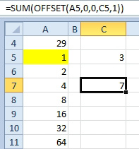
In this case, use =SUM(OFFSET(A5,0,0,C5,1)).

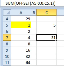
The numbers 1, 2, 4, 8, 16, 32, 64 are in A5:A11. Cell C5 says 5. If you ask for OFFSET(A5,0,0,C5,1) you will get a range five cells tall starting at A5. Send that into the SUM and you get 31. — Figure 487. This formula sums A5:A9.

Change the 5 in C5 to a 3, and the formula sums A5:A7.

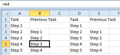
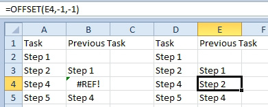
Change the 5 to a 3 and the OFFSET function now refers to a range that is 3 rows tall. — Figure 488. Change C5 to a 3, and the sum range resizes.

OFFSET can be used to point to one cell above the current cell. Why would you go to that hassle when a simple formula does the same thing?

Cell B5 says =A4. Simple enough. — Figure 489. Who needs OFFSET when =A4 works?

What happens when you delete row 4? The simple formula in column B changes to a #REF! error. The OFFSET formula in column E continues to work.

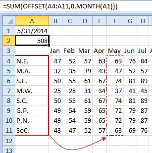
Someone deletes a row and the old formula changes to #REF!. Another way: In E4, use =OFFSET(E4,-1,-1). — Figure 490. If rows might be deleted, OFFSET saves the day.

Additional Details: The starting range can be more than one cell. In the example that follows, the starting range is A4:A11. The third argument of the OFFSET function uses MONTH(A1) to move five columns to the right. This formula will total the column corresponding to the date in cell A1.

Another way to use OFFSET. Months Jan, Feb, Mar stretch across B3:M3. A date in A1 says May 31. OFFSET(A4:A11,0,MONTH(A1) will point five columns to the right, or May. — Figure 491. Use OFFSET to move a range n columns to the right.

Gotcha: OFFSET is a volatile function. This means that with every calculation of the worksheet, the OFFSET is recalculated, even if none of the cells in the table changed. Those cells could stay the same for a whole month, yet OFFSET will recalculate every time that you change a cell anywhere in this worksheet. Many OFFSET functions can cause your worksheet to slow down. In many cases, you can use INDEX instead.

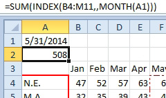
Back in the VLOOKUP topics, you read how to use =INDEX( B4:M11,row,column) to return one cell from a range. If you leave out the row argument blank, Excel will return all of the rows. The formula of =SUM(INDEX(B4:M11,,MONTH(A1))) will return an equivalent result.

=SUM(INDEX(B4:M11,,MONTH(A1)). By leaving the second argument for INDEX is blank, it will return the whole column. — Figure 492. Leave the Row argument of INDEX blank to return an entire column.

This article is an excerpt from Power Excel With MrExcel

Title photo by Volodymyr Hryshchenko on Unsplash