
Sum Visible Rows
March 09, 2021 - by Bill Jelen

Challenge: A SUM function totals all the cells in a range, whether they are hidden or not. You want to sum only the visible rows.
Solution: You can use the SUBTOTAL function instead of SUM. The formula you need is slightly different, depending on how you hid the rows.
If rows are hidden by using Format, Row, Hide, you use:
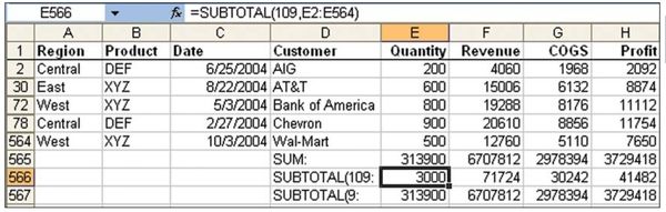
=SUBTOTAL(109, E2:E564)
This is an unusual use for SUBTOTAL. Normally, SUBTOTAL is used to force Excel to ignore other SUBTOTAL cells within a range. SUBTOTAL can perform
any of 11 operations. The first parameter indicates Average (1), Count (2), CountA (3), Max (4), Min (5), Product (6), StdDev (7), StdDevP (8), Sum (9), Var (10), or VarP (11). When you add 100 to this parameter, Excel includes only visible cells in the result.
In Figure 42, you can see that the result of the SUM in row 565 and the result of the SUBTOTAL(9, in row 567 are identical. When you switch to SUBTOTAL(109,in row 566, Excel total only the visible cells in the range.
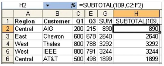
Gotcha: There is an error in Excel Help. The Help topic says that the 100 series parameters sum only visible cells. This is true only of cells that are in hidden rows. If your data is hidden due to hiding a column, Excel still includes those cells (Figure 43).
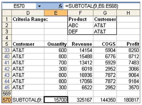
Additional Details: There is an unusual exception to the behavior of the SUBTOTAL function. When your rows have been hidden by any of the Filter commands (Advanced Filter, AutoFilter, or Filter), Excel includes only the visible rows in a SUBTOTAL(9,function. There is no need to use the 109 version. In Figure 44, Advanced Filter is used to find only the AT&T records for two products. The regular SUBTOTAL with an argument of 9 works fine to sum only the visible rows.
Why even mention this strange anomaly? Because there is a little-known shortcut key to sum the visible rows as the result of a filter. Try these steps:
- Choose one cell in your data set.
- From the Excel 2003 menu, choose Data, Filter, AutoFilter. From the Excel 2007 ribbon, choose Data, Filter. Excel adds dropdowns to each heading.
- Open the Customer dropdown. In Excel 2003, choose one customer. In Excel 2007, uncheck Select All and then choose one customer.
- Move the cell pointer to a cell immediately below the filtered data. Choose a cell below one or all of the numeric columns.
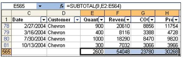
- Press Alt+= or click the AutoSum icon. Instead of using a
SUMfunction, Excel uses=SUBTOTAL(9,which totals only the rows selected by the filter (Figure 45).
Tip: After adding the formulas shown in Figure 45, insert two blank rows above row 1. Cut the formulas in the total row and paste to the new row 1. After you do this, your ad hoc totals are always visible near the headings.
Summary: You can use variations of the SUBTOTAL function to ignore hidden rows.
Title Photo: Ruslan Bardash at Unsplash.com
This article is an excerpt from Excel Gurus Gone Wild.