Switching Columns into Rows Using a Formula

May 23, 2022 - by Bill Jelen

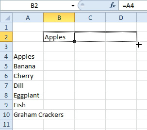
Problem: Every day, I receive a file with information going down the rows. I need to use formulas to pull this information into a horizontal table. It is not practical for me to use Paste Special, Transpose every day. Below, you can see that the first formula in B2 points to A4. If I drag this formula to the right, there is no way that it will pull values from A5, A6, A7, and so on.

A list of 7 products starting in A4 to A10. You want to transpose with a formula. Start with =A4 in cell B2. When you drag to the right, it will not work. — Figure 483. Dragging the fill handle will fail here.

Strategy: You can use the INDEX function to return the nth item from the A4:A10 range. It would be cool if there were a function that could return the numbers 1, 2, 3, and so on as you copy across.

The formula =COLUMN(A1) will return a 1 to indicate that cell A1 is in the first column. While this is not entirely amazing, the beautiful thing about this function is that as you copy to the right, =COLUMN(A1) will change to =COLUMN(B1) and return a 2. Any time you need to fill in the numbers 1, 2, 3 as you go across a row, you can use the =COLUMN(A1) in the first cell. As you copy, Excel will take care of the rest.

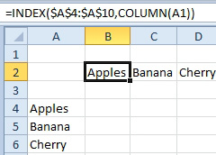
Therefore, if you use the formula =INDEX($A$4:$A$10,COLUMN(A1)) in cell B2, you can easily copy it across the columns.

Gotcha: You need to use A1 as the reference for the COLUMN function no matter where you are entering the formula. In this example, the first formula is in column B. That is irrelevant. Even if the formula starts in column XFA, you will still point to A1 in order to return the number 1.

Instead, use =INDEX($A$4:$A$10,COLUMN(A1)) and drag to the right. — Figure 484. Copy B2 across to transpose with a formula.

Alternate Strategy: It is slightly harder to use, but the TRANSPOSE function will perform the same task as COLUMN. The trick is that a single function has to be entered in many cells at once. Follow these steps:

1. Count the number of cells in A4:A10. In this case, it is seven cells.
2. Select seven horizontal cells. In this case, select B2:H2.
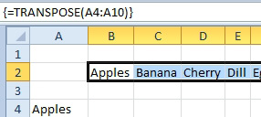
3. Type =TRANSPOSE(A4:A10). Unlike INDEX, dollar signs are not necessary in this formula. Do not press Enter.
4. Because this function will return many answers, you have to hold down Ctrl+Shift while you press Enter. Excel will add curly braces around the function, and the seven values will appear across your selection.

Or - select 7 horizontal cells. Type =TRANSPOSE(A4:A10) and press Ctrl+Shift+Enter. — Figure 485. A single TRANSPOSE function fills in these cells.

The advantage of using TRANSPOSE over using Paste Special, Transpose is that the TRANSPOSE function is a live formula. If cells in column A change, they will change in row 2.

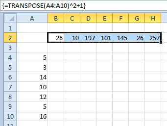
Additional Details: The example in this topic is a trivial example of merely copying the cells. In real life, you might need to do calculations instead of copying the data. You can use calculations with either the INDEX or TRANSPOSE functions. For example, the formula shown above squares the number and adds 1.

If you had 7 numbers in A4:A10 and you wanted to both transpose and transform, you could use =TRANSPOSE(A4:A10)^2+1) followed by Ctrl+Shift+Enter. — Figure 486. Do calculations while transposing.

This article is an excerpt from Power Excel With MrExcel

Title photo by Possessed Photography on Unsplash