Understand Implicit Intersection

January 28, 2022 - by Bill Jelen

In the previous article, Why use the intersection operator, notice that the formulas in the last two figures were outside of the range B:I. Before Dynamic Arrays are introduced to Office 365, those formulas would not work in that area due to a feature called “Implicit Intersection”. Here is how it works.

The named range ProdF runs from B7:I7. Before Dynamic Arrays, if you enter a formula anywhere in columns B through I and that formula references ProdF, you will only get the value from that column of ProdF. In the image below, a formula of =ProdF in E11 returns the 20 from cell E7. Once Dynamic Arrays were introduced, you now have to tell Excel that you really want to use Implicit Intersection, so the formula becomes =@ProdF.

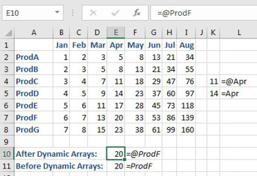
This clearly is not intuitive. In my Power Excel seminars, I occasionally find people who are taking advantage of the formula, but few are doing it knowingly. In a similar fashion, a formula of =Apr anywhere in rows 2:8 will return only the April sales from that row. After Dynamic Arrays, you would have to use =@Apr to call out implicit intersection.

This feels like the old Natural Language Formulas in Excel 2003, but it is a different feature.

This article is an excerpt from Power Excel With MrExcel

Title photo by pan xiaozhen on Unsplash