
Up/Down Markers
August 18, 2017 - by Bill Jelen

Icon Sets debuted in Excel 2007
There is a super-obscure way to add up/down markers to a pivot table to indicate an increase or a decrease.
Somewhere outside the pivot table, add columns to show increases or decreases. In the figure below, the difference between I6 and H6 is 3, but you just want to record this as a positive change. Asking for the SIGN(I6-H6) will provide either +1, 0, or -1.
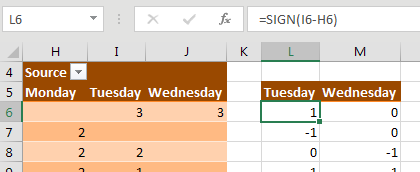
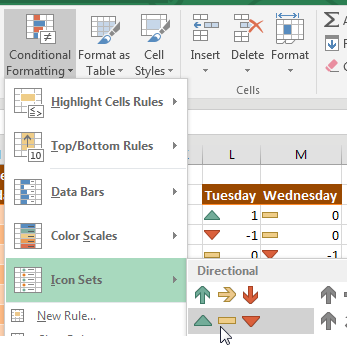
Select the two-column range showing the sign of the change and then select Home, Conditional Formatting, Icon Sets, 3 Triangles. (I have no idea why Microsoft called this option Three Triangles, when it is clearly Two Triangles and a Dash.)
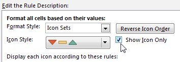
With the same range selected, now select Home, Conditional Formatting, Manage Rules, Edit Rule. Check the Show Icon Only checkbox.
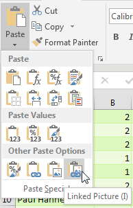
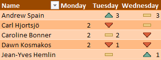
With the same range selected, press Ctrl + C to copy. Select the first Tuesday cell in the pivot table. From the Home tab, open the Paste Dropdown and choose Linked Picture. Excel pastes a live picture of the icons above the table.
At this point, adjust the column widths of the extra two columns showing the icons so that the icons line up next to the numbers in your pivot table.
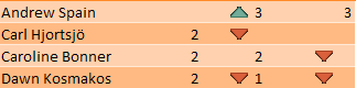
After seeing this result, I don't really like the thick yellow dash to indicate “no change”. If you don't like it either, select Home, Conditional Formatting, Manage Rules, Edit. Open the dropdown for the thick yellow dash and choose No Cell Icon.
Watch Video
- Icon Sets debuted in Excel 2007
- In Excel 2010, they added a set with Up, Flat, Down
- But an icon set can only look at one cell! How can you use it to compare two cells?
- Copy two helper columns off to the side
- Use a calculation to show the change
- Type that formula without using the mouse or arrow keys to prevent =GETPIVOTDATA
- Use the SIGN function to convert that to +1, 0, -1
- Add the Three Triangles icon set to the helper cells
- Why do they call it Three Triangles, when it is really 2 triangles and a dash?
- Manage Rules, Edit the Rule. Show Icon Only.
- Manage Rules, Edit the Rule. Change from percent to numbers
- Use > 0 for Green up arrow
- Use >=0 for yellow dash
- all of the negative numbers will get the red down arrow
- Copy the column widths from the original cells to the helper cells using Paste Special Column Widths
- Copy the Helper Cells
- Paste Linked Picture (this used to be the camera tool)
- Turn off the gridlines with View, Gridlines
- If you don't like the yellow dash for "No Change", manage rules, edit the rule, use No Cell Icon
- To force the camera tool to update, click the camera tool. Click in the Formula Bar. Press Enter
Video Transcript
Learn Excel from MrExcel Podcast, Episode 2007 -- Up/down Markers
I'll be podcasting this entire book. Click that I on the top right-hand corner to subscribe.
Welcome back to the Mr.Excel in that cast I'm Bill Jelen. This is not one of the 40 tips in the book. It's one of the bonus tips between the other tips, because after showing yesterday's podcast of how to compare three lists, I said boy it would be really nice if we had some indicator if we were up or down, and so Conditional Formatting icon sets came along in Excel 2007, but not all of these. They added a few of them in Excel 2010 and one that I remember that they added to Excel 2010 was this one, that they call 3 Triangles.
We just look at it, it's not three triangles at all, it's two triangles in a dash, anyway. This indicates up/down or flat but how the heck are we supposed to use this because icon sets can't look at any other cells. They only look at the cell where the icon appears, so it doesn't know if it's up or down. So here is my crazy trick that I use for this. I'm going to copy these headings out here to be helper cells, alright. And here I'm going to build a formula that is =M7-L7.
Now why did I type that instead of using the mouse or arrow keys? Because I don't want get Pivot Data to happen, Alright, so I'm going to copy that formula, all the way throughout like this. Bam. Actually, probably even the grand totals too. Yep, okay now that gives me a wide variety of numbers. Plus 3, minus 2, zero. I need this to be three numbers. Either it was up, it was down, it was negative, or it was flat, which is 0.
So I'm going to use the sine function but not the one from trigonometry not sine, SIGN says we're going to do that math and then it's either so they're going to be minus 1 for negative, 0 for 0, or plus 1 for positive. Alright, that's beautiful.
Now here in the Helper Cells, we're going to do Conditional Formatting, Icon Sets, 3 Triangles, also known as two triangles in a ash, and we get our indicator showing whether we're up flat or down. Now, I need to get rid of the numbers, so Conditional Formatting, Manage Rules, Edit the Rule and say, show icon only. That also is brand new in Excel 2010 and see, and that gives us now an arrow up, arrow down, or flat.
In real life, we would have built this way out there, off the right-hand side of the screen, so no one else would ever see it. We're going to copy these cells, Ctrl C. We're going to come here in our Pivot Table. I want the indicators to show up on Tuesday or Wednesday and we're going to do something really cool. Paste a linked picture, a linked picture. Now in order to make this work, this column width, has to be the same as this column width. So I'm going to copy these two columns, Ctrl C and then come over here I'm going to use paste special and paste the column widths and it's almost good, except for what we're seeing in the grid lines. So let's just turn the grid lines off. I could come out here and get rid, yeah, let's just turn the gridlines off. Make it look better.
You know and now that I look at this, I'm not a big fan of the the big yellow dashed indicate flat, so back here, select all of these, Home, Conditional Formatting, Manage Rules, Edit the Rule and we're going to say No Cell Icon for the center one. Click OK, click OK.
Alright, now if there was ever a weird case where everything was down, there were no ups at all and all you had was zeros and ones; then you definitely might want to come in and take the extra time to manage these rules, Edit the Rule, change this from percent to number, percent to number, where it's greater than. It say, if it's greater than zero you get this. If it was greater than, or equal to zero, no cell icon and then everything less than zero will get the down arrow.
Right? But provided you have a mix of increases and decreases, the other way is probably save. I take that back. Now it's not safe. Always to take the extra time to make sure, because sooner or later there's going to be someone where you know everyone bails out and all the Euros and Rupees are down and you don't have any ups. So go ahead and take the extra time to do that.
Also, did you notice that the the camera tool wasn't updating here. This is another bug. Oh man, so I'm on the first release programs. That means I get new bits, but for some reason that wasn't updating. I selected the camera tool, came here and just pressed Enter and that seemed to force it to recalc. I don't know what's up with that. Very bizarre.
Anyway, this bonus tip, 40 real tips, plus a whole bunch of bonus tips, plus other stuff is in this book. Go buy the book, ten bucks for an e-book, twenty-five bucks for the real book. It's in color, lots of fun stuff here.
Alright episode recap: Icon Sets, they debuted in Excel 2007 but it was 2010 when they added the set with up, flat and down, but how can you use the compare to cells, because the icon can only look at one cell? Created to helper columns, off to the side, use a calculation to show the change and then converted that calculation, using the sign SIGN function to make it plus 1 zero and minus 1. Add the 3 Triangles. Why do they call it 3 Triangles? When it's really two triangles and a dash. Edit the Rule. Use greater than zero for the green up arrow, greater than or equal to zero for the yellow dash, all the negative members will get the red arrow. You want to copy the column widths from the original cells to the helper cells. I did that with paste special column widths. Copy those helper cells. Paste this link picture. It's down under the paste drop down/ It used to be called the camera tool. Turn off the grid lines with view gridlines and then maybe take out the dash. Manage Rules, Edit Rule use No Cell Icon for the dash.
The camera tool didn't update, so I had to click the Camera Tool, click in the Formula Bar and press Enter to get its updates.
Hey I want to thank you for stopping by all. See you next time for another netcast from MrExcel.
Download File
Download the sample file here: Podcast2007.xlsx
Title Photo: geralt / pixabay