
Use A Self-referencing Formula
March 31, 2021 - by Bill Jelen

Challenge: Shades was looking for a formula to reverse letters in a cell. This can easily be accomplished using a VBA function. However, Shades had challenged people to write a formula. A new member, Hady, came along with this solution.
Gotcha: The technique in this topic is not compatible with the Evaluate Formula feature. If you use Evaluate Formula on a self-referencing formula, you run the risk of crashing Excel and losing your work.
Solution: To solve this problem, you use a self-referencing formula. Follow these steps:
- Select Tools, Options, Calculation. Choose Iteration and set the maximum iterations to 100.
- Enter any sentence in A1.
- In cell B1, enter this formula and press Enter:
=IF(LEN(B1) < LEN(A1)+1, B1 & MID(A1, LEN(A1) + 1 — LEN (B1), 1), IF(MID(B1, 1, 1) <> "0", B1, RIGHT(B1, LEN(A1)) & " ")), When you press Enter, you get a result of 0 and the last character from cell A1. This is normal. - Press F9 again, and you get 0, the last character, and the second-to-last character.
- Press F9 again, and you get 0 and the last three characters in reverse.
- Keep pressing F9. When you have 0 and all of the characters, press F9 one last time, and the 0 is removed.
- To start over, go to B1, press F2 to put the formula in Edit mode, and press Ctrl + Shift + Enter.
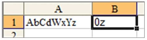
Breaking It Down: Let’s say you put AbCdWxYz in cell A1. When the formula starts, the value of B1 is 0. The LEN of A1 is 8, and the LEN of B1 is 0, so the formula takes whatever is in B1 and concatenates it with the MID of A1. The MID function says to start at the character that is the LEN of A1 minus the LEN of B1 + 1. In the first calculation, this appends the starting 0 with the final character, and you will have 0z in cell B1 (Figure 59).
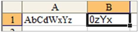
As the result in B1 gets longer, the formula keeps appending characters further from the end of A1. After you press F9 a few more times, you have 0zY in B1. The LEN of A1 is still 8. The LEN of B1 is 3. You are using 8+1 – 3, so you are now asking for the sixth character to be appended to B1, and you now get 0zYx in B1, as shown in Figure 60.
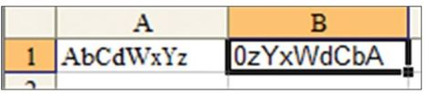
You eventually get to the point where you have a 0 and the complete text from A1, in reverse, as shown in Figure 61.
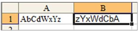
The formula finally gets to use the last part of the formula, where it takes the RIGHT characters from B1, this time grabbing only the LEN of A1. This strips out the leading 0, as shown in Figure 62.
Additional Details: Although this formula can do something VBA-like without using any VBA, it has limited use. You cannot copy the formula down to any other cells. And if you change A1, you need to start over and press F9 a bunch of times.
However, it is an interesting technique, and there have been a few instances at the MrExcel message board where Hady’s approach was suggested:
- Fill in a DOT after each character
- June/July 2008 Challenge of the Month
- FORMULA CHALLENGE shortest wins!
Summary: You can use a self-referencing formula to replace a VBA user-defined function.
Source: CHALLENGE (and Ramblings on Palindromes) on the MrExcel Message Board.
The post was nominated by Andrew Fergus.
Title Photo: Reinhart Julian on Unsplash
This article is an excerpt from Excel Gurus Gone Wild.