Use Get Cell To Highlight Non-formula Cells

February 05, 2021 - by Bill Jelen

Challenge: You want to highlight all the cells on a worksheet that do not contain formulas.

Solution: Before VBA, macros were written in an old macro language now known as XLM. That language offered a GET. CELL function, which provides far more information than the current CELL function. In fact, GET. CELL can tell you more than five dozen different attributes of a cell.

GET. CELL is cool, but there is one gotcha. You cannot enter this function directly in a cell. You have to define a name to hold the function and then refer to the name in the cell. For example, to find out whether cell A1 contains a formula, you use =GET. CELL (48, Sheet1!A1). However, you need something more generic than this for the conditional formatting formula. Using =INDIRECT (“RC”, FALSE) is a handy way to refer to the cell in which the formula exists. Thus, the formula to tell if the current cell contains a formula is:

=GET.CELL(48, INDIRECT("RC", FALSE))

To make use of this formula, follow these steps in Excel 2003:

To define a new name, select Insert, Name Define and use a suitable name, such as Has Formula. In the Refers To box, type =GET.CELL (48, INDIR ECT (“RC”, FALSE) ) , as shown in Figure 18. Click Add. Click OK. You use the Define Name dialog to define a name in Excel 2003.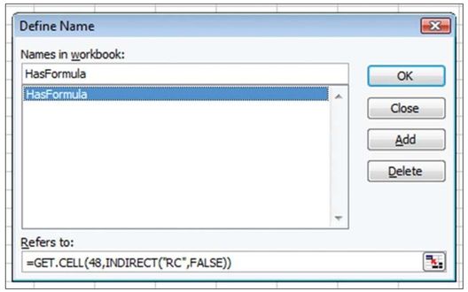

Figure 18. You use the Define Name dialog to define a name in Excel 2003.
Select a range of cells.
Select Format, Conditional Formatting. Change the first dropdown to Formula Is. Type =HASFORMULA, as shown in Figure 19. Click the Format button and choose a format for the cell. Click OK.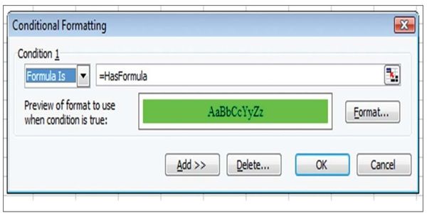

Figure 19. You can use the relatively obscure Formula Is version of conditional formatting.

To make use of this formula, follow these steps in Excel 2007:

To define a new name, select Formulas, Name Manager, New and use a suitable name, such as HasFormula. In the Refers To box, type =GET. CEL L (48, INDIRECT (“RC”, FALSE) ) , as shown in Figure 20. Click OK. Click Close. You use the New Name dialog to define a name in Excel 2007.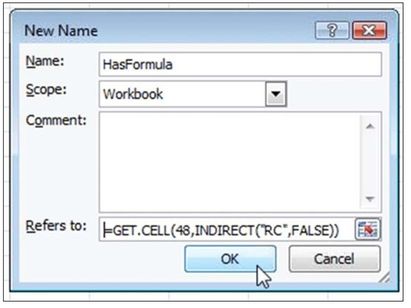

Figure 20. You use the New Name dialog to define a name in Excel 2007.
Select the cells to which you want to apply the conditional formatting.
Select Home, Conditional Formatting, New Rule. Choose Use a Formula to Determine Which Cells to Format. In the lower half of the dialog type =HASFORMULA, as shown in Figure 21. Click the Format button and choose a format for the cell. Click OK.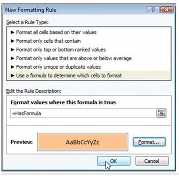

Figure 21. You use the New Formatting Rule dialog to set up conditional formatting in Excel 2007.

To highlight every cell that does not contain a formula, use =NOT(HasFormula) in the conditional formatting dialog.

Massive Gotcha: You cannot copy any cells that contain this formula to a different worksheet without risking an Excel crash.

Breaking It Down: While most people typically use A1-style references, the R1C1-style reference works better in the INDIRECT function. Normally, an R1C1-style reference points to another cell. For example, =RC[-2] refers to the current row and two cells to the left of the current cell. =R[10]C[3] refers to 10 rows below and 3 columns to the right of the current cell. An R1C1 formula without any modifiers, =RC, refers to the current cell. This is a case where an R1C1 formula is far simpler than the equivalent A1 formula, =ADDRESS(ROW(), COLUMN(), 4).

Alternate Strategy: The advantage of using the method described above is that the formatting will automatically update whenever someone changes a cell to contain either a formula or a constant. If you simply need to get a snapshot of which cells contain formulas, follow these steps:

Select all cells by pressing Ctrl+A.
Press Ctrl+G to display the Go To dialog.
Click the Special button in the lower-left corner of the Go To dialog.
In the Go To Special dialog, choose Formulas and click OK.
Choose a color from the Paint Bucket icon.

Additional Details: The complete list of GET. CELL arguments follows. Note that in some cases, functionality has changed significantly, and the argument may no longer return valid values.

Argument	Returns
1	Absolute reference of the upper-left cell in reference, as text in the current workspace reference style (usually A1 style, but it might be R1C1 style if someone has chosen R1C1 style in their Excel Options dialog).
2	Row number of the top cell in the reference.
3	Column number of the leftmost cell in the reference.
4	Same as TYPE(reference).
5	Contents of the reference.
6	Formula in the reference, as text, in either A1 or R1C1 style, depending on the workspace setting.
7	Number format of the cell, as text (for example, “m/d/yy” or “General”).
8	Number indicating the cell’s horizontal alignment:
	1 = General
	2 = Left
	3 = Center
	4 = Right
	5 = Fill
	6 = Justify
	7 = Center across cells
9	Number indicating the left-border style assigned to the cell:
	0 = No border
	1 = Thin line
	2 = Medium line
	3 = Dashed line
	4 = Dotted line
	5 = Thick line
	6 = Double line
	7 = Hairline
10	Number indicating the right-border style assigned to the cell. See argument 9 for descriptions of the numbers returned.
11	Number indicating the top-border style assigned to the cell. See argument 9 for descriptions of the numbers returned.
12	Number indicating the bottom-border style assigned to the cell. See argument 9 for descriptions of the numbers returned.
13	Number from 0 to 18, indicating the pattern of the selected cell, as displayed in the Patterns tab of the Format Cells dialog box, which appears when you choose the Cells command from the Format menu. If no pattern is selected, returns 0.
14	If the cell is locked, returns `TRUE`; otherwise, returns `FALSE`.
15	If the cell’s formula is hidden, returns `TRUE`; otherwise, returns `FALSE`.
16	A two-item horizontal array containing the width of the active cell and a logical value that indicates whether the cell’s width is set to change as the standard width changes (`TRUE`) or is a custom width (`FALSE`).
17	Row height of cell, in points.
18	Name of font, as text.
19	Size of font, in points.
20	If all the characters in the cell, or only the first character, are bold, returns `TRUE`; otherwise, returns `FALSE`.
21	If all the characters in the cell, or only the first character, are italic, returns `TRUE`; otherwise, returns `FALSE`.
22	If all the characters in the cell, or only the first character, are underlined, returns `TRUE`; otherwise, returns `FALSE`.
23	If all the characters in the cell, or only the first character, are struck through, returns `TRUE`; otherwise, returns `FALSE`.
24	Font color of the first character in the cell, as a number in the range 1 to 56. If font color is automatic, returns 0.
25	If all the characters in the cell, or only the first character, are outlined, returns `TRUE`; otherwise, returns `FALSE`. Outline font format is not supported by Microsoft Excel for Windows.

26	If all the characters in the cell, or only the first character, are shadowed, returns `TRUE`; otherwise, returns `FALSE`. Shadow font format is not supported by Microsoft Excel for Windows.
27	Number indicating whether a manual page break occurs at the cell:
	0 = No break
	1 = Row
	2 = Column
	3 = Both row and column
28	Row level (outline).
29	Column level (outline).
30	If the row containing the active cell is a summary row, returns `TRUE`; otherwise, returns `FALSE`.
31	If the column containing the active cell is a summary column, returns `TRUE`; otherwise, returns `FALSE`.
32	Name of the workbook and sheet containing the cell. If the window contains only a single sheet that has the same name as the workbook, without its extension, returns only the name of the book, in the form BOOK1.XLS. Otherwise, returns the name of the sheet, in the form [Book1]Sheet1.
33	If the cell is formatted to wrap, returns `TRUE`; otherwise, returns `FALSE`.
34	Left-border color, as a number in the range 1 to 56. If color is automatic, returns 0.
35	Right-border color, as a number in the range 1 to 56. If color is automatic, returns 0.
36	Top-border color, as a number in the range 1 to 56. If color is automatic, returns 0.
37	Bottom-border color, as a number in the range 1 to 56. If color is automatic, returns 0.
38	Shade foreground color, as a number in the range 1 to 56. If color is automatic, returns 0.
39	Shade background color, as a number in the range 1 to 56. If color is automatic, returns 0.
40	Style of the cell, as text.
41	Returns the formula in the active cell without translating it. (This is useful for international macro sheets.)
42	The horizontal distance, measured in points, from the left edge of the active window to the left edge of the cell. May be a negative number if the window is scrolled beyond the cell.
43	The vertical distance, measured in points, from the top edge of the active window to the top edge of the cell. May be a negative number if the window is scrolled beyond the cell.
44	The horizontal distance, measured in points, from the left edge of the active window to the right edge of the cell. May be a negative number if the window is scrolled beyond the cell.
45	The vertical distance, measured in points, from the top edge of the active window to the bottom edge of the cell. May be a negative number if the window is scrolled beyond the cell.
46	If the cell contains a text note, returns `TRUE`; otherwise, returns `FALSE`.
47	If the cell contains a sound note, returns `TRUE`; otherwise, returns `FALSE`.
48	If the cells contains a formula, returns `TRUE`; if a constant, returns `FALSE`.
49	If the cell is part of an array, returns `TRUE`; otherwise, returns `FALSE`.
50	Number indicating the cell’s vertical alignment:
	1 = Top
	2 = Center
	3 = Bottom
	4 = Justified
51	Number indicating the cell’s vertical orientation:
	0 = Horizontal
	1 = Vertical
	2 = Upward
	3 = Downward
52	The cell prefix (or text alignment) character, or empty text (“”) if the cell does not contain one.
53	Contents of the cell as it is currently displayed, as text, including any additional numbers or symbols resulting from the cell’s formatting.
54	Returns the name of the PivotTable view containing the active cell.
55	Returns the position of a cell within the PivotTable view.
56	Returns the name of the field containing the active cell reference if inside a PivotTable view.
57	Returns `TRUE` if all the characters in the cell, or only the first character, are formatted with a superscript font; otherwise, returns `FALSE`.
58	Returns the font style as text of all the characters in the cell, or only the first character, as displayed in the Font tab of the Format Cells dialog box (for example, “Bold Italic”.)
59	Returns the number for the underline style:
	1 = None
	2 = Single
	3 = Double
	4 = Single accounting
	5 = Double accounting
60	Returns `TRUE` if all the characters in the cell, or only the first character, are formatted with a subscript font; otherwise, returns `FALSE`.
61	Returns the name of the PivotTable item for the active cell, as text.
62	Returns the name of the workbook and the current sheet, in the form [book1]sheet1.
63	Returns the fill (background) color of the cell.
64	Returns the pattern (foreground) color of the cell.
65	Returns `TRUE` if the Add Indent alignment option is on (Far East versions of Microsoft Excel only); otherwise, returns `FALSE`.
66	Returns the book name of the workbook containing the cell in the form BOOK1.XLS.

Summary: You can use GET. CELL to return more information than is available by using the CELL function. You can then use conditional formatting to highlight every cell that does not contain a formula.

Source: Info only - get.cell arguments on the MrExcel Message Board.

Title Photo: Patrick Tomasso at Unsplash.com

This article is an excerpt from Excel Gurus Gone Wild.