
VLOOKUP with Multiple Results
January 15, 2018 - by Bob Umlas

Examine this figure:
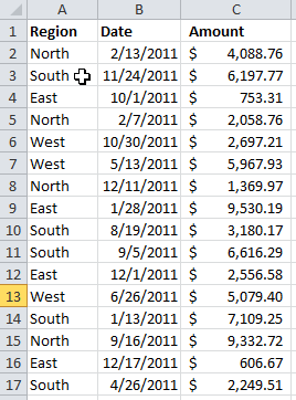
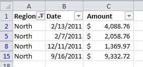
Suppose you want to produce a report from this as if you filtered on the Region. That is, if you filter on North, you would see:
But what if you wanted a formula-based version of the same thing?
Here’s the result you are looking for in columns I:K:
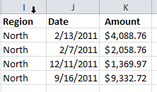
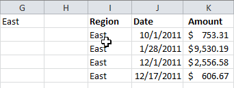
Clearly, it’s the same report, but there are no filtered items here. If you wanted a new report on East, it’d be nice to simply change the value in G1 to East:
Here’s how it’s done. First of all, it’s not done using VLOOKUP. So I lied about the title of this technique!
Column F was not shown before, and it can be hidden (or moved somewhere else so it doesn’t interfere with the report).
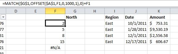
What’s shown in column F is the row numbers of where G1 is found in column A; that is, what rows contain the value “North”? This technique involves using the cell above, so it must begin in at least row 2. It matches the value “North” against column A, but instead of the entire column, use an OFFSET function: OFFSET($A$1,F1,0,1000,1).
Since F1 is 0, this is OFFSET(A1,0,0,1000,1) which is A1:A1000. (The 1000 is arbitrary, but large enough to do the job – you can make it any other number).
The value 2 in F2 is where the first “North” is. You also want to add back the value of F1 at the end, but this is zero, so far.
The “magic” comes to life in in cell F3. You already know that the first North is found in Row 2. So, you want to start searching two rows below A1. You can do that by specifying 2 as the second argument of the OFFSET function.
The formula in F3 will automatically point to the 2 that was calculated in cell F2: When you copy the formula down, you will see =OFFSET($A$1,F2,0,1000,1) which is OFFSET($A$1,2,0,1000,1)which is A3:A1000. So you are matching North against this new range and it finds North in the third cell of this new range, so the MATCH gives 3.
By adding back the value from the cell above, F2, you will see the 3 plus the 2, or 5, which is the row which contains the second North.
This formula is filled down far enough to get all the values.
That will get you the row numbers where all of the North records are found.
How do you translate those row numbers to the results in columns I through K? It is all done with a single formula. Enter this formula in I2: =IFERROR(INDEX(A:A,$F2),””). Copy right and then copy down.
Why use IFERROR? Where’s the error? Notice cell F6 – it contains #N/A (which is why you would want to hide column F) because there are no more North’s after row 15. So if column F is an error, return a blank. Otherwise pick up the value from column A (and when filled right, B & C).
The $F2 is an absolute reference to column F so the fill right still refers to column F.
Title Photo: Matúš Kovačovský / Unsplash

This guest article is from Excel MVP Bob Umlas. It is one of his favorite techniques from his book, Excel Outside the Box.