How to plot this data

[excelos]

Hello

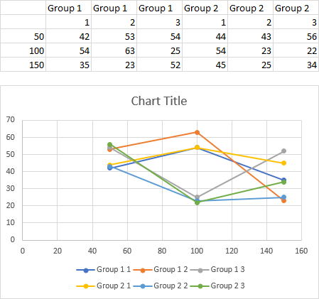
I have a data like this:

Group 1
1 2 3
50 42 53 54
100 54 63 25
150 35 23 52


Group 2
1 2 3
50 44 43 56
100 54 23 22
150 45 25 34

etc

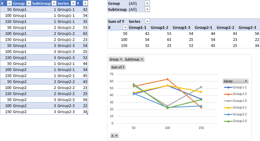
I want to plot in one graph the lines:
Group1-1
Group1-2
Group1-3
Group2-1
Group2-2
Group2-3

all versus 50,100,150

How can I do this please instead of manually adding each line? They are so many it will take too much time.

Thanks!

 

[Jon Peltier]

Rearrange your data like shown below. Note the two blank cells in the first column.

Select the range, then insert an XY Scatter Chart. You will probably have to switch rows and columns, because I had to. Excel likes to plot fewer series with more points.

 

[excelos]

Rearrange your data like shown below. Note the two blank cells in the first column.

Select the range, then insert an XY Scatter Chart. You will probably have to switch rows and columns, because I had to. Excel likes to plot fewer series with more points.

thanks, it didnt work like that exactly, I had to name the columns Group1-1, Group1-2, Group2-1, etc for it to work.

Now how do I select which lines/sets to display? I want to be able to select by filtering the names of the lines/sets, but I can't find a way. Because the lines/sets are many, I cannot just scroll through the list and tick/untick them.

Is there any solution for this? I was wondering if Pivot can help, but I can't make it work.

Thanks!

 

[excelos]

Anyone???

 

[Jon Peltier]

So how do you want to filter the series? Show or Hide all of Group1 or Group2, for example? Show or Hide all like GroupX-1 or GroupX-2?

Set up your data as in the table below left. The data is the same as in your first post, but the Series column has a formula that concatenates the Group1 and the subgroup number with a hyphen.

Then make a pivot table, with Group and Subgroup in the Filters area, Series in the Columns area, X in the Rows area, and Y (or Sum of Y) in the Values area. Then make a chart.

Now you can filter the fields in the Filters area easily to show and hide large blocks of data. Below I've filtered Group so that only Group1 shows (Group1-1, Group1-2, and Group1-3 are visible).

Below I've filtered Subgroups so that only 1 and 3 appear in the pivot table and chart (Group1-1, Group1-3, Group2-1, and Group2-3 are visible).

 

[Jon Peltier]

Note that a pivot chart cannot be an XY chart. In the case of your sample data, it doesn't matter, since 50, 100, and 150 are evenly spaced. If you actually needed an XY chart, you would have to do some other trickery to make it work.

You can Make Regular Charts from Pivot Tables, but the regular charts will not update their source range as nicely as a pivot chart: when you filter the pivot table, the chart will still include empty series from the blank cells that contained data before you filtered it.