Data labels on the outside end of error bars without overlapping?

Crucis · Aug 31, 2017

Dear all,

I have a recurrent problem when making column/bar charts with error bars and data labels. Whenever I add data labels to the outside end, these labels will always overlap the error bars (please see image). Is there any automatic solution to position the data labels on the outside end of the error bars (instead of the column end)? Dragging each data label manually is annoying and time consuming when dealing with a lot of data.

Thanks in advance for your help!

Crucis · Sep 11, 2017

Hey Phil,

I have just tested it and this last piece of code knocked it out of the park! Thank you very much!!!

Huey72 · Nov 6, 2019

Hi Phil - your solution is from a very old post, but it looks like it will completely solve my problem...have been struggling with this for days. My data is structured differently however, and I haven't been successful in adjusting the code to run from my data structure vs. the data being in the 4 columns as specified. Wondering if you'd be willing to guide me through modifying your code to meet my specific needs? Thanks is advance - very much appreciated!

Steve

pbornemeier · Nov 6, 2019

Post a few rows of your data here and explain how it is incorporated into your graph and I will see if I can figure it out.

Huey72 · Nov 6, 2019

Thanks so much Phil, I really appreciate it!

I use an Excel table named tblMyData as the data source for the chart. In the Chart, organizations H6 and H7 have their data label '*' overlapped by the custom high error bar. I'm hoping to use a version of your code to place the label above the high error bar.

The listcolumns I use for the chart are: Organization, Stratification, Plot Value, High Error Bar, and Data Label. Overall, this fits into a solution that creates ~150 charts * 20 organizations and makes a PowerPoint report for each of the organizations - this was a defect that came up in testing and I'm struggling to solve for it.

Excel 2016 (Windows) 64 bit

	[COLOR=[URL=https://www.mrexcel.com/forum/usertag.php?do=list&action=hash&hash=FFFFFF]#FFFFFF[/URL] ]CC[/COLOR]	[COLOR=[URL=https://www.mrexcel.com/forum/usertag.php?do=list&action=hash&hash=FFFFFF]#FFFFFF[/URL] ]CF[/COLOR]	[COLOR=[URL=https://www.mrexcel.com/forum/usertag.php?do=list&action=hash&hash=FFFFFF]#FFFFFF[/URL] ]CG[/COLOR]	[COLOR=[URL=https://www.mrexcel.com/forum/usertag.php?do=list&action=hash&hash=FFFFFF]#FFFFFF[/URL] ]CH[/COLOR]	[COLOR=[URL=https://www.mrexcel.com/forum/usertag.php?do=list&action=hash&hash=FFFFFF]#FFFFFF[/URL] ]CJ[/COLOR]	[COLOR=[URL=https://www.mrexcel.com/forum/usertag.php?do=list&action=hash&hash=FFFFFF]#FFFFFF[/URL] ]CK[/COLOR]	[COLOR=[URL=https://www.mrexcel.com/forum/usertag.php?do=list&action=hash&hash=FFFFFF]#FFFFFF[/URL] ]CL[/COLOR]	[COLOR=[URL=https://www.mrexcel.com/forum/usertag.php?do=list&action=hash&hash=FFFFFF]#FFFFFF[/URL] ]CM[/COLOR]	[COLOR=[URL=https://www.mrexcel.com/forum/usertag.php?do=list&action=hash&hash=FFFFFF]#FFFFFF[/URL] ]CN[/COLOR]	[COLOR=[URL=https://www.mrexcel.com/forum/usertag.php?do=list&action=hash&hash=FFFFFF]#FFFFFF[/URL] ]CO[/COLOR]	[COLOR=[URL=https://www.mrexcel.com/forum/usertag.php?do=list&action=hash&hash=FFFFFF]#FFFFFF[/URL] ]CP[/COLOR]	[COLOR=[URL=https://www.mrexcel.com/forum/usertag.php?do=list&action=hash&hash=FFFFFF]#FFFFFF[/URL] ]CQ[/COLOR]	[COLOR=[URL=https://www.mrexcel.com/forum/usertag.php?do=list&action=hash&hash=FFFFFF]#FFFFFF[/URL] ]CR[/COLOR]	[COLOR=[URL=https://www.mrexcel.com/forum/usertag.php?do=list&action=hash&hash=FFFFFF]#FFFFFF[/URL] ]CS[/COLOR]	[COLOR=[URL=https://www.mrexcel.com/forum/usertag.php?do=list&action=hash&hash=FFFFFF]#FFFFFF[/URL] ]CU[/COLOR]	[COLOR=[URL=https://www.mrexcel.com/forum/usertag.php?do=list&action=hash&hash=FFFFFF]#FFFFFF[/URL] ]CV[/COLOR]	[COLOR=[URL=https://www.mrexcel.com/forum/usertag.php?do=list&action=hash&hash=FFFFFF]#FFFFFF[/URL] ]CW[/COLOR]	[COLOR=[URL=https://www.mrexcel.com/forum/usertag.php?do=list&action=hash&hash=FFFFFF]#FFFFFF[/URL] ]CY[/COLOR]	[COLOR=[URL=https://www.mrexcel.com/forum/usertag.php?do=list&action=hash&hash=FFFFFF]#FFFFFF[/URL] ]CZ[/COLOR]	[COLOR=[URL=https://www.mrexcel.com/forum/usertag.php?do=list&action=hash&hash=FFFFFF]#FFFFFF[/URL] ]DA[/COLOR]	[COLOR=[URL=https://www.mrexcel.com/forum/usertag.php?do=list&action=hash&hash=FFFFFF]#FFFFFF[/URL] ]DF[/COLOR]	[COLOR=[URL=https://www.mrexcel.com/forum/usertag.php?do=list&action=hash&hash=FFFFFF]#FFFFFF[/URL] ]DG[/COLOR]	[COLOR=[URL=https://www.mrexcel.com/forum/usertag.php?do=list&action=hash&hash=FFFFFF]#FFFFFF[/URL] ]DH[/COLOR]	[COLOR=[URL=https://www.mrexcel.com/forum/usertag.php?do=list&action=hash&hash=FFFFFF]#FFFFFF[/URL] ]DI[/COLOR]	[COLOR=[URL=https://www.mrexcel.com/forum/usertag.php?do=list&action=hash&hash=FFFFFF]#FFFFFF[/URL] ]DJ[/COLOR]
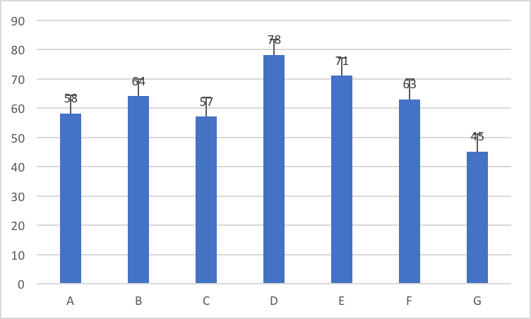
[COLOR=[URL=https://www.mrexcel.com/forum/usertag.php?do=list&action=hash&hash=FFFFFF]#FFFFFF[/URL] ]1[/COLOR]	[COLOR=[URL=https://www.mrexcel.com/forum/usertag.php?do=list&action=hash&hash=FFFFFF]#FFFFFF[/URL] ]Period[/COLOR]	[COLOR=[URL=https://www.mrexcel.com/forum/usertag.php?do=list&action=hash&hash=FFFFFF]#FFFFFF[/URL] ]Organization[/COLOR]	[COLOR=[URL=https://www.mrexcel.com/forum/usertag.php?do=list&action=hash&hash=FFFFFF]#FFFFFF[/URL] ]Indicator[/COLOR]	[COLOR=[URL=https://www.mrexcel.com/forum/usertag.php?do=list&action=hash&hash=FFFFFF]#FFFFFF[/URL] ]Stratification[/COLOR]	[COLOR=[URL=https://www.mrexcel.com/forum/usertag.php?do=list&action=hash&hash=FFFFFF]#FFFFFF[/URL] ]Volume[/COLOR]	[COLOR=[URL=https://www.mrexcel.com/forum/usertag.php?do=list&action=hash&hash=FFFFFF]#FFFFFF[/URL] ]Observed Rate[/COLOR]	[COLOR=[URL=https://www.mrexcel.com/forum/usertag.php?do=list&action=hash&hash=FFFFFF]#FFFFFF[/URL] ]Expected Rate[/COLOR]	[COLOR=[URL=https://www.mrexcel.com/forum/usertag.php?do=list&action=hash&hash=FFFFFF]#FFFFFF[/URL] ]Adjusted Rate[/COLOR]	[COLOR=[URL=https://www.mrexcel.com/forum/usertag.php?do=list&action=hash&hash=FFFFFF]#FFFFFF[/URL] ]Lower 95% CI[/COLOR]	[COLOR=[URL=https://www.mrexcel.com/forum/usertag.php?do=list&action=hash&hash=FFFFFF]#FFFFFF[/URL] ]Higher 95% CI[/COLOR]	[COLOR=[URL=https://www.mrexcel.com/forum/usertag.php?do=list&action=hash&hash=FFFFFF]#FFFFFF[/URL] ]Low Error Bar[/COLOR]	[COLOR=[URL=https://www.mrexcel.com/forum/usertag.php?do=list&action=hash&hash=FFFFFF]#FFFFFF[/URL] ]High Error Bar[/COLOR]	[COLOR=[URL=https://www.mrexcel.com/forum/usertag.php?do=list&action=hash&hash=FFFFFF]#FFFFFF[/URL] ]Median[/COLOR]	[COLOR=[URL=https://www.mrexcel.com/forum/usertag.php?do=list&action=hash&hash=FFFFFF]#FFFFFF[/URL] ]90th Percentile[/COLOR]	[COLOR=[URL=https://www.mrexcel.com/forum/usertag.php?do=list&action=hash&hash=FFFFFF]#FFFFFF[/URL] ]Plot value >5[/COLOR]	[COLOR=[URL=https://www.mrexcel.com/forum/usertag.php?do=list&action=hash&hash=FFFFFF]#FFFFFF[/URL] ]Plot value <=5[/COLOR]	[COLOR=[URL=https://www.mrexcel.com/forum/usertag.php?do=list&action=hash&hash=FFFFFF]#FFFFFF[/URL] ]Plot value[/COLOR]	[COLOR=[URL=https://www.mrexcel.com/forum/usertag.php?do=list&action=hash&hash=FFFFFF]#FFFFFF[/URL] ]25th Percentile[/COLOR]	[COLOR=[URL=https://www.mrexcel.com/forum/usertag.php?do=list&action=hash&hash=FFFFFF]#FFFFFF[/URL] ]75th Percentile[/COLOR]	[COLOR=[URL=https://www.mrexcel.com/forum/usertag.php?do=list&action=hash&hash=FFFFFF]#FFFFFF[/URL] ]Mean[/COLOR]	[COLOR=[URL=https://www.mrexcel.com/forum/usertag.php?do=list&action=hash&hash=FFFFFF]#FFFFFF[/URL] ]MAX[/COLOR]	[COLOR=[URL=https://www.mrexcel.com/forum/usertag.php?do=list&action=hash&hash=FFFFFF]#FFFFFF[/URL] ]Data Label[/COLOR]	[COLOR=[URL=https://www.mrexcel.com/forum/usertag.php?do=list&action=hash&hash=FFFFFF]#FFFFFF[/URL] ]Num[/COLOR]	[COLOR=[URL=https://www.mrexcel.com/forum/usertag.php?do=list&action=hash&hash=FFFFFF]#FFFFFF[/URL] ]Max Scale[/COLOR]	[COLOR=[URL=https://www.mrexcel.com/forum/usertag.php?do=list&action=hash&hash=FFFFFF]#FFFFFF[/URL] ]Values Axis Minor Unit[/COLOR]
[COLOR=[URL=https://www.mrexcel.com/forum/usertag.php?do=list&action=hash&hash=FFFFFF]#FFFFFF[/URL] ]2[/COLOR]	2016/17	H1	1-Year All-Cause Mortality Following PCI	Emergent PCI	1745	0.118995633	0.1045545	0.12	0.1028	0.1363	0.0162	0.0173			0.12		0.12				0.0373		22	0.2	0.05
[COLOR=[URL=https://www.mrexcel.com/forum/usertag.php?do=list&action=hash&hash=FFFFFF]#FFFFFF[/URL] ]3[/COLOR]	2016/17	H2	1-Year All-Cause Mortality Following PCI	Emergent PCI	315	0.159722222	0.124679127	0.13	0.095	0.1741	0.039	0.0401			0.13		0.13				0.0601		22	0.2	0.05
[COLOR=[URL=https://www.mrexcel.com/forum/usertag.php?do=list&action=hash&hash=FFFFFF]#FFFFFF[/URL] ]4[/COLOR]	2016/17	H3	1-Year All-Cause Mortality Following PCI	Emergent PCI	506	0.103139013	0.103062158	0.11	0.0704	0.1399	0.0346	0.0349			0.11		0.11				0.0549		22	0.2	0.05
[COLOR=[URL=https://www.mrexcel.com/forum/usertag.php?do=list&action=hash&hash=FFFFFF]#FFFFFF[/URL] ]5[/COLOR]	2016/17	H4	1-Year All-Cause Mortality Following PCI	Emergent PCI	628	0.074074074	0.095905428	0.08	0.0495	0.1127	0.0316	0.0316			0.08		0.08				0.0516		22	0.2	0.05
[COLOR=[URL=https://www.mrexcel.com/forum/usertag.php?do=list&action=hash&hash=FFFFFF]#FFFFFF[/URL] ]6[/COLOR]	2016/17	H5	1-Year All-Cause Mortality Following PCI	Emergent PCI	0																0.05		22	0.2	0.05
[COLOR=[URL=https://www.mrexcel.com/forum/usertag.php?do=list&action=hash&hash=FFFFFF]#FFFFFF[/URL] ]7[/COLOR]	2016/17	H6	1-Year All-Cause Mortality Following PCI	Emergent PCI	357	0.14	0.106783462	0.14	0.0957	0.1797	0.0413	0.0427			0.14		0.14				0.0627	*	22	0.2	0.05
[COLOR=[URL=https://www.mrexcel.com/forum/usertag.php?do=list&action=hash&hash=FFFFFF]#FFFFFF[/URL] ]8[/COLOR]	2016/17	H7	1-Year All-Cause Mortality Following PCI	Emergent PCI	997	0.113924051	0.091444649	0.13	0.1054	0.1563	0.0246	0.0263			0.13		0.13				0.0463	*	22	0.2	0.05
[COLOR=[URL=https://www.mrexcel.com/forum/usertag.php?do=list&action=hash&hash=FFFFFF]#FFFFFF[/URL] ]9[/COLOR]	2016/17	H8	1-Year All-Cause Mortality Following PCI	Emergent PCI	683	0.096209913	0.119217925	0.08	0.0584	0.1111	0.0264	0.0263			0.08		0.08				0.0463		22	0.2	0.05

Sheet: PCI 1 year mortality

pbornemeier · Nov 7, 2019

I would guess that the desired graph is a column chart (similar to first chart in this thread) with the organization labels on the horizontal axis, plot values as vertical columns, low/high error bars bracketing the top of each column. I am not sure of the placement of the stratification items.

This code is a streamlined subset of the previous code based on what I understand you are asking for and the above assumptions.

Code:

Option Explicit

Sub MoveAndEditDataLabels()

    Dim cht As Chart
    Dim ser As Series
    Dim rngSeries As Range
    Dim sFormula As String
    Dim lDLOffset As Long
    Dim rngDL As Range
    Dim lHEOffset As Long
    Dim rngHE As Range
    Dim pt As Point
    Dim sngX As Single
    Dim sngY As Single
    Dim sngColumnHeight As Single
    Dim sngScalingFactor As Single
    Dim lMaxPoint As Long
    Dim aryValues As Variant
    Dim aryDataLabels As Variant
    Dim aryErrors As Variant
    Dim sngMaxValue As Single
    Dim lPointIndex As Long
    Dim lPointCount As Long
    Dim sngValue As Single
    
    'Edit if your current setup changes
    Set cht = ActiveSheet.ChartObjects(1).Chart     'Replace 1 with your chart's index or name
    Set ser = cht.SeriesCollection("Plot Value")    'Edit if required
    lDLOffset = 5 'Relationship between CS and CX   'Edit if required
    lHEOffset = -5 'Relationship between CS and CN  'Edit if required
    
    sFormula = Split(ser.Formula, ",")(2)           'Get location of plot values
    Set rngSeries = Range(Split(sFormula, "!")(1))  'convert to range
    Set rngDL = rngSeries.Offset(0, lDLOffset)      'Get range of desired data labels
    Set rngHE = rngSeries.Offset(0, lHEOffset)      'Get range of High Error values
    
    aryValues = Range(rngSeries.Address)
    aryDataLabels = Range(rngDL.Address)
    aryErrors = Range(rngHE.Address)

    'Reset the data labels to their original position before applying correction
    If ser.HasDataLabels Then ser.HasDataLabels = False
    ser.HasDataLabels = True
    ser.DataLabels.Position = xlLabelPositionOutsideEnd
    
    'Calculate Offset Scaling Factor based on tallest column
    sngMaxValue = 0
    lPointCount = ser.Points.Count
    For lPointIndex = 1 To lPointCount
        sngValue = aryValues(lPointIndex, 1)
        If sngValue > sngMaxValue Then
            sngMaxValue = sngValue
            lMaxPoint = lPointIndex
        End If
    Next
    sngColumnHeight = ser.Points(lMaxPoint).Height
    sngScalingFactor = sngColumnHeight / sngMaxValue
    
    'Move & Edit Labels
    For lPointIndex = 1 To lPointCount
        With ser.Points(lPointIndex).DataLabel
            If Not IsEmpty(aryErrors(lPointIndex, 1)) Then
                .Top = .Top - (aryErrors(lPointIndex, 1) * sngScalingFactor) + 5
                .Text = aryDataLabels(lPointIndex, 1)
            End If
        End With
    Next

End Sub

Huey72 · Nov 7, 2019

Thanks Phil - the desired graph is a clustered column chart. The stratification column includes the series labels. There are 3 stratification's/series: Emergent PCI, Non-Emergent PCI, and Total PCI.

Yes, the organization labels are on the horizontal axis, plot values as vertical columns, and low/high error bars bracketing the top of each column. I'm new to the board - still trying to figure out how to include a screen shot for you, in case that helps.

When I run the code, I get a parameter not valid error on this line:
Set ser = cht.SeriesCollection("Plot value") 'Edit if required

pbornemeier · Nov 8, 2019

To post an image, upload it to an image sharing site then use IMG tags around the link to include it in your post:
[IMG]https://cdn3.iconfinder.com/data/icons/developerkit/png/Ball%20Red.png[/IMG]
I used the NOPARSE tags on the above line so the BB code for posting an image would NOT be processed. The following image is referenced by using the line that you see above.

More image posting guidance can be found here:
https://www.mrexcel.com/forum/misc.php?do=bbcode#imgcode

Regarding:

Code:

Set ser = cht.SeriesCollection("Plot value") 'Edit if required

I used "Plot Value" as the name of the series that held the CS column in your data, It determines the height of the columns in my version of your graph.
If your graph must have a different name for that series, so change "Plot Value" to the names of that series (keep the double quotes on each end)

I cannot get the data as presented to cluster. Are you doing some intermediate processing to get the clustered graph?
Please run this code and post the output from the immediate window in the VBE. It will help me understand how your data is laid out and how to modify the code to work with it. (Or at least allow me to ask questions from a less ignorant position).

Code:

Sub DocumentSeries()

    Dim ser As Series
    Dim lSeriesIndex As Long
    
    'Select a chart then run this code
    If Not ActiveChart Is Nothing Then
        'A chart is selected
        Debug.Print "Start Series Documentation =============================="
        For Each ser In ActiveChart.SeriesCollection
            Debug.Print ser.PlotOrder
            Debug.Print ser.Name
            Debug.Print ser.Formula
        Next
        Debug.Print "End Series Documentation ================================"
    Else
        MsgBox "Select a chart then run this code"
    End If

End Sub

Huey72 · Nov 8, 2019

Thanks again Phil - I'll go to the test area for the site and practice posting HTML, images, and attachments to make it easier to share information, sorry for causing any confusion.

The sample records I provided didn't include the other two data series - it only has sample records from the first stratification...I think I should have provide data that illustrated each of the three series. I think your series documentation code will help to clarify the sample.

Start Series Documentation ==============================
1
Total PCI
=SERIES("Total PCI",'PCI 30 Day Mortality'!$O$38:$O$55,'PCI 30 Day Mortality'!$AE$2:$AE$19,1)
2
Emergent PCI
=SERIES("Emergent PCI",'PCI 30 Day Mortality'!$O$38:$O$55,'PCI 30 Day Mortality'!$AE$20:$AE$37,2)
3
Non-Emergent PCI
=SERIES("Non-Emergent PCI",'PCI 30 Day Mortality'!$O$38:$O$55,'PCI 30 Day Mortality'!$AE$38:$AE$55,3)
End Series Documentation ================================

Should also note - in an effort to simplify (which I don't think I did very well) in my description and the series documentation above, I consolidated the data into one table and re-built the chart off of that. In reality, because this is part of a bigger solution which creates hundreds of charts from a larger data source, I use the advanced filter functionality to create each data series for the chart in it's own table. In a more accurate view of how it actually works, here's what the output of the series documentation based on that:

Start Series Documentation ==============================
1
Total PCI
=SERIES("Total PCI",tblMyData_TotalPCI[Organization],tblMyData_TotalPCI[Plot value],1)
2
Emergent PCI
=SERIES("Emergent PCI",tblMyData_EmergentPCI[Organization],tblMyData_EmergentPCI[Plot value],2)
3
Non-Emergent PCI
=SERIES("Non-Emergent PCI",tblMyData_NonEmergentPCI[Organization],tblMyData_NonEmergentPCI[Plot value],3)
End Series Documentation ================================

I hope that helps - thank you again!

pbornemeier · Nov 8, 2019

I modified the code to work with the series definitions in the first part of your last post.
You have to edit these lines to reflect the layout of you data

Code:

    lDLOffset = 5 'Column relationship between Y-Values and Data Label columns
    lHEOffset = -5 'Column relationship between Y-Values and High Error

Code:

Sub EditAndMoveDataLabel()

    Dim cht As Chart
    Dim ser As Series
    Dim rngSeries As Range
    Dim sFormula As String
    Dim rngDL As Range
    Dim rngHE As Range
    Dim pt As Point
    Dim sngX As Single
    Dim sngY As Single
    Dim sngColumnHeight As Single
    Dim sngScalingFactor As Single
    Dim lMaxPoint As Long
    Dim aryValues As Variant
    Dim aryDataLabels As Variant
    Dim aryErrors As Variant
    Dim sngMaxValue As Single
    Dim lPointIndex As Long
    Dim lPointCount As Long
    Dim sngValue As Single
    Dim lSerIndex As Long
    Dim lDLOffset As Long   'The relative position of the Data Label column from the Y-Values column
    Dim lHEOffset As Long   'The relative position of the High Error column from the Y-Values column
                            '-1 would be one column to the left, 4 would be four columns to the right
    
    'For the original sample data, CS held the Y-Values, CX held the Data labels and
    '  CN held the High Error values.  So the relationship between the columns was:
    lDLOffset = 5 'Column relationship between Y-Values and Data Label columns
    lHEOffset = -5 'Column relationship between Y-Values and High Error
    'Edit the above numbers to match the current column relationships
    
    'Extra steps are required if the series formulas use named range or table references.
        
    Set cht = ActiveSheet.ChartObjects(1).Chart     'If more than one chart on the activesheet
                                                    '  replace 1 with your chart's index or name
    
    For lSerIndex = 1 To cht.SeriesCollection.Count
    
        Set ser = cht.SeriesCollection(lSerIndex)
        
        'Split function creates a 0..n array of the text value in the first argument divided by the
        '  single text character in the second argument
        sFormula = Split(ser.Formula, ",")(2)           'Get location of plot values as text
        
        'Sample sFormula layout example for column chart series:
        '=SERIES("Plot Value",Sheet1!$CD$3:$CF$40,Sheet1!$CS$3:$CS$40,1)            'SERIES Formula
        '         Name       ,X-Axis (Category)  ,Y-Axis (Value)     ,Plot Order    'Formula Part Names
        '         0           1                   2                   3             'Split Array Index
        
        Set rngSeries = Range(Split(sFormula, "!")(1))  'Get range of Y-Axis cells
        Set rngDL = rngSeries.Offset(0, lDLOffset)      'Get range of desired Data Labels
        Set rngHE = rngSeries.Offset(0, lHEOffset)      'Get range of High Error values
        
        aryValues = Range(rngSeries.Address)            'Get values for each point
        aryDataLabels = Range(rngDL.Address)            'Get desired Data Labels for each point
        aryErrors = Range(rngHE.Address)                'Get high error values for each point
    
        'Reset the data labels to their original position before applying correction
        If ser.HasDataLabels Then ser.HasDataLabels = False
        ser.HasDataLabels = True
        ser.DataLabels.Position = xlLabelPositionOutsideEnd
        
        'Calculate Offset Scaling Factor based on tallest column
        sngMaxValue = 0
        lPointCount = ser.Points.Count
        For lPointIndex = 1 To lPointCount
            sngValue = aryValues(lPointIndex, 1)
            If sngValue > sngMaxValue Then
                sngMaxValue = sngValue
                lMaxPoint = lPointIndex
            End If
        Next
        sngColumnHeight = ser.Points(lMaxPoint).Height
        sngScalingFactor = sngColumnHeight / sngMaxValue
        
        'Move & Edit Labels
        For lPointIndex = 1 To lPointCount
            With ser.Points(lPointIndex).DataLabel
                If Not IsEmpty(aryErrors(lPointIndex, 1)) Then
                    .Top = .Top - (aryErrors(lPointIndex, 1) * sngScalingFactor - 3)
                    .Text = aryDataLabels(lPointIndex, 1)
                End If
            End With
        Next
        
    Next

End Sub

Which of the layouts in your last post should be used to construct the code to move the data labels?
For each series involved, the code has to "know" the location of 3 ranges:
1) range that contains the vertical value of the column
2) range that contains the positive errors
3) range that contains the new data labels

If any range specification uses named ranged or table references then the above code will required some changes. Let me know if that is the case or if the above code does not work as desired.

This was the series documentation for the graph I tested:

Start Series Documentation ==============================
1
A
=SERIES("A",Sheet1!$CF$17:$CF$23,Sheet1!$CS$3:$CS$9,1)
2
B
=SERIES("B",Sheet1!$CF$17:$CF$23,Sheet1!$CS$10:$CS$16,2)
3
C
=SERIES("C",Sheet1!$CF$17:$CF$23,Sheet1!$CS$17:$CS$23,3)
End Series Documentation ================================

Huey72 · Nov 8, 2019

This is amazing Phil - for the series documentation you tested, this works like a charm. The real structure of the data as you noted is the second version, where each of the three data series are in three different data tables...it follows this series documentation:

Start Series Documentation ==============================
1
Total PCI
=SERIES("Total PCI",tblMyData_TotalPCI[Organization],tblMyData_TotalPCI[Plot value],1)
2
Emergent PCI
=SERIES("Emergent PCI",tblMyData_EmergentPCI[Organization],tblMyData_EmergentPCI[Plot value],2)
3
Non-Emergent PCI
=SERIES("Non-Emergent PCI",tblMyData_NonEmergentPCI[Organization],tblMyData_NonEmergentPCI[Plot value],3)
End Series Documentation ================================

In my code I reference the three tables using : .ListObjects("tblMyData_TotalPCI"), .ListObjects("tblMyData_EmergentPCI"), and .ListObjects("tblMyData_NonEmergentPCI")
and I reference the columns using : .ListColumns("Organization").DataBodyRange, .ListColumns("Plot value").DataBodyRange, .ListColumns("High Error Bar").DataBodyRange, and .ListColumns("Data Label").DataBodyRange

I hope that makes sense - let me know if any questions - thanks so much!!

Data labels on the outside end of error bars without overlapping?

Crucis

New Member

Crucis

New Member

Excel Facts

Huey72

New Member

pbornemeier

Well-known Member

Huey72

New Member

pbornemeier

Well-known Member

Huey72

New Member

pbornemeier

Well-known Member

Huey72

New Member

pbornemeier

Well-known Member

Huey72

New Member

Similar threads

Forum statistics

Share this page

Data labels on the outside end of error bars without overlapping?

New Member

New Member

Excel Facts

New Member

Well-known Member

New Member

Well-known Member

New Member

Well-known Member

New Member

Well-known Member

New Member

Similar threads

Forum statistics

Share this page

We've detected that you are using an adblocker.

Which adblocker are you using?

Disable AdBlock

Disable AdBlock Plus

Disable uBlock Origin

Disable uBlock