Sort columns in an array so each column has either a blank or a duplicate value

Kinkzor

New Member
Joined
Feb 14, 2018
Messages
3
Hi all,

Little hard to explain, I Will add an image to show the sort of array I am working on:
3adoAMQ.jpg


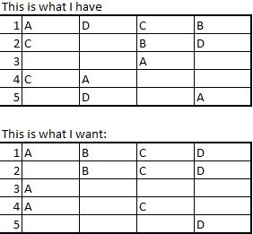
So each column contains omly the duplicate values. Each row will contain the letters correlating to each number, with blanks if that number has no link to a specific letter.
 

Excel Facts

Best way to learn Power Query?
Read M is for (Data) Monkey book by Ken Puls and Miguel Escobar. It is the complete guide to Power Query.
How to identify what should go in each column? In your case it's letters from A to D so it can be done as per below. But how is it in your real scenario?


<b>Worksheet Formulas</b><table cellpadding="2.5px" width="100%" rules="all" style="border: 1px solid;text-align:center;background-color: rgb(255,255,255);border-collapse: collapse; border-color: rgb(187,187,187)"><thead><tr style=" background-color: rgb(218,231,245);color: rgb(22,17,32)"><th width="10px">Cell</th><th style="text-align:left;padding-left:5px;">Formula</th></tr></thead><tbody><tr><th width="10px" style=" background-color: rgb(218,231,245);color: rgb(22,17,32)">B9</th><td style="text-align:left">=IF(<font color="Blue">ISNUMBER(<font color="Red">MATCH(<font color="Green">CHAR(<font color="Purple">MOD(<font color="Teal">COLUMNS(<font color="#FF00FF">$B:B</font>)-1,26</font>)+65</font>),$B1:$E1,0</font>)</font>),CHAR(<font color="Red">MOD(<font color="Green">COLUMNS(<font color="Purple">$B:B</font>)-1,26</font>)+65</font>),""</font>)</td></tr></tbody></table></td></tr></table><br />


Excel 2010
ABCDE
11ADCB
22CBD
33A
44CA
55DA
6
7
8
91ABCD
102BCD
113A
124AC
135AD
Sheet17
 
Upvote 0
Hi and thanks for the reply.

Each row is a department, the columns are filled with application names used in each department. Some departments have 1 or 2 apps used some have 50.

App names are typical such as office 2016 or vba dev and so on.
 
Upvote 0
so I guess you will need to make a mapping of the apps that would need to go in each column and then update the formula accordingly. remove the part where it creates the letter name CHAR(MOD(COLUMNS($B:B)-1,26)+65) and replace it with the app name
 
Upvote 0
so I guess you will need to make a mapping of the apps that would need to go in each column and then update the formula accordingly. remove the part where it creates the letter name CHAR(MOD(COLUMNS($B:B)-1,26)+65) and replace it with the app name

Hi VBA Geek, thanks for the reply.

The issue is i have in the real sheet around 900 different application names and 300+ departments (we are a large company).

I could take all apps, remove duplicates, make this new list the top row and then tell excel to compare an entire row with the value at the top row, and if it finds it.. print a "Yes".

This way I would eventually have a top row of app names, left column of departments, with a "Yes" in each square where the app is used.

Make sense? This should work, I will give it a shot now, thanks!
 
Upvote 0

Forum statistics

Threads
1,214,968
Messages
6,122,506
Members
449,089
Latest member
RandomExceller01

We've detected that you are using an adblocker.

We have a great community of people providing Excel help here, but the hosting costs are enormous. You can help keep this site running by allowing ads on MrExcel.com.
Allow Ads at MrExcel

Which adblocker are you using?

Disable AdBlock

Follow these easy steps to disable AdBlock

1)Click on the icon in the browser’s toolbar.
2)Click on the icon in the browser’s toolbar.
2)Click on the "Pause on this site" option.
Go back

Disable AdBlock Plus

Follow these easy steps to disable AdBlock Plus

1)Click on the icon in the browser’s toolbar.
2)Click on the toggle to disable it for "mrexcel.com".
Go back

Disable uBlock Origin

Follow these easy steps to disable uBlock Origin

1)Click on the icon in the browser’s toolbar.
2)Click on the "Power" button.
3)Click on the "Refresh" button.
Go back

Disable uBlock

Follow these easy steps to disable uBlock

1)Click on the icon in the browser’s toolbar.
2)Click on the "Power" button.
3)Click on the "Refresh" button.
Go back
Back
Top