need help with a formula

[djs6025]

Hi Everybody,
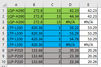
I'm looking for a formula to look at duplicates in column A and return the lowest # in column D from those duplicates. I also need it to ignore the cells with "#N/A". The answer & formula will be in column E. Hopefully, I've explain that well enough. Below is a link to a screen shot I took for what I'm looking for. Thanks so much for your help.


https://imgur.com/a/Rp2Bc


Thanks,
Dan

 

[cerfani]

the correct link is https://i.imgur.com/vaoXTDI.png

 

[cerfani]

maybe

{=MIN(IFERROR(IF(A:A=A1,D:D,9999999999),99999999))}

untested, this is an array formula you would drag down next to the table... It would look for all matches in column A on the corresponding Row and retrieve the value in column D and if not found it will use a large number as a placeholder since we will be looking for the lowest value... if it sees that the value in D is N/A it will just replace it with a large number to use in the min formula. Maybe it will work for you. Also you dont want to reference an entire column so edit the ranges to the size of the table

There is a way to type the largest excel number in scientific notation but a bunch of 9s should work too

 

[djs6025]

Unfortunately, this formula didn't work. Here are the results it gave me: https://imgur.com/a/wGN6C

 

[jtakw]

Hi,

If you want the #N/A error from Column D to show in Column E, use formula in E1 copied down, if you Don't want it to show use F1 formula:

Book1
	A	B	C	D	E	F
1	LQP-H260	272.8	13	42.23	42.23	42.23
2	LQP-H260	272.8	13	44.34	42.23	42.23
3	LQP-H260	272.8	13	#N/A	#N/A	42.23
4	LTP-L330	420.36	3	56.22	53.29	53.29
5	LTP-L330	420.36	3	53.29	53.29	53.29
6	LTP-L330	420.36	3	54.78	53.29	53.29
7	LTP-L330	420.36	3	#N/A	#N/A	53.29
8	LLP-P210	132.68	2	20.26	20.26	20.26
9	LLP-P210	132.68	2	23.38	20.26	20.26
10	LLP-P210	132.68	2	23.34	20.26	20.26
Sheet10

Cell Formulas
Range	Formula
E1	{=IF(ISERROR(D1),D1,MIN(IF(ISNUMBER(D$1:D$10),IF(A$1:A$10=A1,D$1:D$10))))}
F1	{=MIN(IF(ISNUMBER(D$1:D$10),IF(A$1:A$10=A1,D$1:D$10)))}
Press CTRL+SHIFT+ENTER to enter array formulas.

 

[djs6025]

Unfortunately, I couldn't get that to work either. Here are the results I got: https://imgur.com/a/OxNgy

 

[jtakw]

Unfortunately, I couldn't get that to work either. Here are the results I got: https://imgur.com/a/OxNgy

Please read the instructions in my post, you NEED to enter the either one of the formulas by Control-Shift-Enter.

 

[jtakw]

If you had copied and pasted my formulas into your sheet, remove the curly brackets { }, then hold down Control-Shift and hit Enter, Excel will add the { }.

 

[djs6025]

It worked! Thank you so much! You saved me from doing this manually on a 14k line spreadsheet. You're a lifesaver.

Thanks,
Dan

 

[jtakw]

You're welcome, glad you got it working.