BlackYellow
New Member
- Joined
- Mar 22, 2018
- Messages
- 3
Hi everyone,
I have a very difficult, very complex problem.
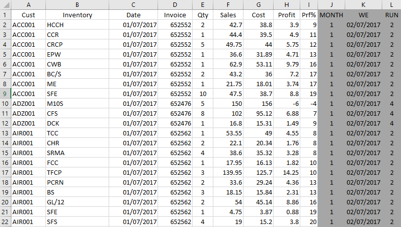
I have a spreadsheet of sales data which looks like this:
The 3 last columns in grey are my own formula to calculate fiscal year, week ending and territory (uses VLOOKUP to repeat data from another sheet)
When I display it on a pivot table, I sum the sales data per Customer, group it by Run (Territory) and sort it by WE (Week Ending).
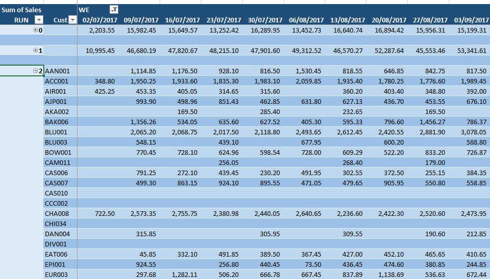
The main purpose of this spreadsheet is to show me the spending patterns of each customer by territory however to see a more accurate reflection of their overall spending over the period of a financial year, I'd need to see their rolling average and how it changes over time.
How would I do this in a pivot table? If not possible in a pivot table, how can I calculate this and display it on a separate sheet?
For example:
If I were to manually calculate rolling average, it would be...
Week 1 Rolling average = Week 1 Sales / Week Number
Week 2 Rolling average = Week 1 Sales + Week 2 Sales / Week Number
Week 3 Rolling average = Week 1 Sales + Week 2 Sales + Week 3 Sales / Week Number
I have a very difficult, very complex problem.
I have a spreadsheet of sales data which looks like this:
The 3 last columns in grey are my own formula to calculate fiscal year, week ending and territory (uses VLOOKUP to repeat data from another sheet)
When I display it on a pivot table, I sum the sales data per Customer, group it by Run (Territory) and sort it by WE (Week Ending).
The main purpose of this spreadsheet is to show me the spending patterns of each customer by territory however to see a more accurate reflection of their overall spending over the period of a financial year, I'd need to see their rolling average and how it changes over time.
How would I do this in a pivot table? If not possible in a pivot table, how can I calculate this and display it on a separate sheet?
For example:
If I were to manually calculate rolling average, it would be...
Week 1 Rolling average = Week 1 Sales / Week Number
Week 2 Rolling average = Week 1 Sales + Week 2 Sales / Week Number
Week 3 Rolling average = Week 1 Sales + Week 2 Sales + Week 3 Sales / Week Number


