Numerical Code Generation Based off of Text from other Columns

[iceshark17]

I have a specific code structure that I would like to be automatically generated based off of text from other columns in the same row.

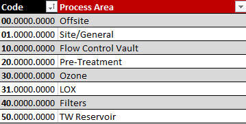
The code Structure is: XX.XXXX.XXXX (PROCESS AREA . COMPONENT/DISCIPLINE . ITEM)

The first two digits are meant to represent an "Area" (##.XXXX.XXXX)

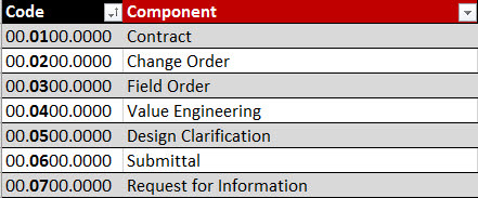
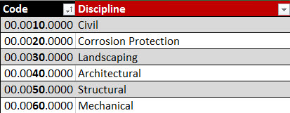
The next four digits are meant to represent a "Component" (XX.##XX.XXXX) as well as a "Discipline" if applicable (XX.XX##.XXX), if not applicable the ##s will just be zeros.

The last four digits will represent an item number, 0001-9999 that will simply follow the order in which the row was entered.

Example of text:

so, for example, I'd like to fill out a row such as the one below with all the text information and have the code automatically generate.

Any guidance would be much appreciated. Thank you!

 

[iceshark17]

Hi Peter,

1. I took the (red & black headed) tables and moved them to be columns within a larger, single table. This is what I meant by saying I tried to combine your method with Mark's.

(FYI I pasted the same image twice, one w color and one black and white in case one was easier to read/follow than the other.)

2. The 'Process Area' Table, for example, moved to columns F & G. The 'Component' table moved to columns H & I. The 'Discipline' Table moved to columns J & K.

3. Thanks, I wasn't sure how so I had just pasted the formula at the end of my last post. I tried downloading the MR. Excel HTML maker and it won't open. I'm on a work machine as well and probably shouldn't tweak any settings, hopefully we can make do with the pasted formula for now.

Thank you

 

[markmzz]

Hi Peter,

1. I took the (red & black headed) tables and moved them to be columns within a larger, single table. This is what I meant by saying I tried to combine your method with Mark's.

(FYI I pasted the same image twice, one w color and one black and white in case one was easier to read/follow than the other.)

2. The 'Process Area' Table, for example, moved to columns F & G. The 'Component' table moved to columns H & I. The 'Discipline' Table moved to columns J & K.

3. Thanks, I wasn't sure how so I had just pasted the formula at the end of my last post. I tried downloading the MR. Excel HTML maker and it won't open. I'm on a work machine as well and probably shouldn't tweak any settings, hopefully we can make do with the pasted formula for now.

Thank you

Hi Iceshark17!

I think that the best approach is with 3 separate tables (not with one table) and with the table labels/headers (not cells address) in the formula. So you can create new codes without problem and you can put the 3 tables in another sheet without problem too.

Here is the formula with 3 tables of codes (the names of the tables are TArea, TComp and TDisc), one table main (the name of the tabel is Main) and with labels (headers) in the formula:

In A2 in the table Main:

=IFERROR(TEXT(INDEX(TArea[Code2],MATCH([@Area],TArea[Process Area],0)),"00"),"00")&"."&
IFERROR(TEXT(INDEX(TComp[Code3],MATCH([@Component],TComp[Component],0)),"00"),"00")&
IFERROR(TEXT(INDEX(TDisc[Code4],MATCH([@[Discipline (if applicable)]],TDisc[Discipline],0)),"00"),"00")&"."&TEXT([@Item],"0000")

A

B

C

D

E

F

G

H

I

J

K

L

M

N

O

1

Code

Area

Component

Discipline (if applicable)

Item

Code2

Process Area

Code3

Component

Code4

Discipline

Description

2

50.0350.0001

TW Reservoir

Field Order

Structural

1

0

Offsite

1

Contract

10

Civil

Staff Gauge

3

31.0560.0002

LOX

Design Clarification

Mechanical

2

1

Site/General

2

Change Order

20

Corrosion Protection

Column Numbering

4

50.0150.0003

TW Reservoir

Contract

Structural

3

10

Flow Control Vault

3

Field Order

30

Landscaping

5 ton weight limit signage

5

31.0300.0004

LOX

Field Order

4

20

Pre-Treatment

4

Value Enginnering

40

Architectural

P&IDs

6

30

Ozone

5

Design Clarification

50

Structural

7

31

LOX

6

Submittal

60

Mechanical

Verify

8

40

Filters

7

Request for Information

9

50

TW Reservoir

*

**************

************

*****************

**********************

*****

*

******

*******************

*

******

**********************

*

******

*********************

***********************

<tbody>
</tbody>

Markmzz

 

[Peter_SSs]

In relation to the HTML maker, you shouldn't be trying to 'Open' it. Some installation instructions are given in post #2 of the thread linked to from the 'Look here' link in my signature block below.

I think that the best approach is with 3 separate tables (not with one table) and with the table labels/headers (not cells address) in the formula.

I agree with Mark & my suggestion is similar, though I interpreted post #1 as saying it was only the "Discipline" column of the result table that could be empty. Perhaps I was wrong about that?

I also agree with Mark that the input tables could go on another sheet if you want but I have included all 4 tables (same names as Mark used) on the one sheet. So below,
Table 'Main' is in columns A:E
Table 'TArea' in cols F:G
Table 'TComp' in cols H:I
Table TDisc' in cols J:K

In practice, you might choose to separate each table by a blank column for better visual clarity.

In your answers to my questions, you didn't address the issue of the 'Code' columns now displaying simple numbers like 30 instead of text like 50.0150.0001 but I will also go with the simple numbers for now. However, to help simplify the formula a bit, I'm suggesting formatting the 'Code' column of each table as Text and then entering the 2-digit code directly. In the TArea table and TDisc table include a "." at the end of each 2-digit number as shown.

For table Main, formulas for Code and Item are shown.

Excel Workbook
	A	B	C	D	E	F	G	H	I	J	K
1	Code	Area	Component	Discipline	Item	Code	Process Area	Code	Component	Code	Discipline
2	50.0150.0001	TW Reservoir	Contract	Structural	:)-1,"0000")]0001	00.	Offsite	01	Contract	10.	Civil
3	20.0660.0002	Pre-Treatment	Submittal	Mechanical	0002	01.	Site/General	02	Change Order	20.	Corrosion Protection
4	31.0300.0003	LOX	Field Order		0003	10.	Flow Control Vault	03	Field Order	30.	Landscaping
5						20.	Pre-Treatment	04	Value Engineering	40.	Architectural
6						30.	Ozone	05	Design Clarification	50.	Structural
7						31.	LOX	06	Submittal	60.	Mechanical
8						40.	Filters	07	Request for Information
9						50.	TW Reservoir
10
Code (3)

 

[iceshark17]

Peter & Mark, thank you very much for your help.

Mark, I separated out the tables on different sheets, applied your formula and got it to work.

Peter, I apologize for being a bit vague in my posts. I did want simple numbers in my reference tables but I had tried to show it in the context of the resulting "Code" which will ultimately be the item's filing number. I tried to use your formula thinking it should work the same as Mark's regardless of where the referenced tables exist within the workbook as I have now referenced them by their table names and not their cells (I had to look up how to name tables so sorry for being slow to catch up). If you could perhaps clarify, am I supposed to be replacing any part of your code after pasting the formula? I tried to replace the '

' portion with '[Code2]' , '[Code3]' , etc..after it had not worked on the first go but I can't tell what else may need to be updated. If it's not apparent, please don't worry as I have something functional at the moment.

Thank you both again you are life savers on this forum.
****** id="cke_pastebin" style="position: absolute; top: 0px; width: 1px; height: 1px; overflow: hidden; left: -1000px;">[TABLE]
<tbody>[TR]
[TD]=INDEX(TArea[Code],MATCH([@Area],TArea[Process Area],0))&INDEX(TComp[Code],MATCH([@Component],TComp[Component],0))&IF(D2="","00.",INDEX(TDisc[Code],MATCH[COLOR=#0000FF]([@Discipline],TDisc[Discipline],0)[/COLOR]))&[@Item][/TD]
[/TR]
</tbody>[/TABLE]
</body>

 

[Peter_SSs]

If you could perhaps clarify, am I supposed to be replacing any part of your code after pasting the formula? I tried to replace the '

' portion with '[Code2]' , '[Code3]' , etc..after it had not worked on the first go but I can't tell what else may need to be updated. If it's not apparent, please don't worry as I have something functional at the moment.[/QUOTE]If you have Mark's working I would just stick with that as mine wasn't a lot different anyway. :)

 

[markmzz]

Peter & Mark, thank you very much for your help.

Mark, I separated out the tables on different sheets, applied your formula and got it to work.

Hi Iceshark17,

You're welcome and thanks for the feedback.

Markmzz