Having no solution about this graph

[alexdodo]

Hello.
I have to do a graph like this:

We have this information:

FROM	TO	DISTANCE
Bucuresti	Craiova	229
Craiova	Timisoara	339
Timisoara	Satu Mare	300
Satu Mare	Botosani	423
Botosani	Bacau	157
Bacau	Constanta	383
Constanta	Ploiesti	282

<tbody>
</tbody>

Can someone explain me how I do this, please?

 

[mole999]

have a search for peltier graphs, tons of graph information there (CHART STUFF) in my Sig

 

[thisoldman]

Have you got Excel 2013 or later?

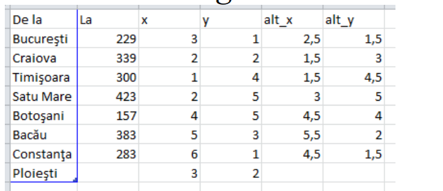
You need the latitudes and longitudes.

<b></b><table cellpadding="2.5px" rules="all" style=";background-color: rgb(255,255,255);border: 1px solid;border-collapse: collapse; border-color: rgb(187,187,187)"><colgroup><col width="25px" style="background-color: rgb(218,231,245)" /><col /><col /><col /><col /></colgroup><thead><tr style=" background-color: rgb(218,231,245);text-align: center;color: rgb(22,17,32)"><th></th><th>A</th><th>B</th><th>C</th><th>D</th></tr></thead><tbody><tr ><td style="color: rgb(22,17,32);text-align: center;">1</td><td style="text-align: right;background-color: #EBEBEB;;"></td><td style="background-color: #EBEBEB;;">Lon</td><td style="background-color: #EBEBEB;;">Lat</td><td style="background-color: #EBEBEB;;">Dist</td></tr><tr ><td style="color: rgb(22,17,32);text-align: center;">2</td><td style=";">Bucuresti</td><td style="text-align: right;;">26.1025</td><td style="text-align: right;;">44.4268</td><td style="text-align: right;;"></td></tr><tr ><td style="color: rgb(22,17,32);text-align: center;">3</td><td style=";">Craiova</td><td style="text-align: right;;">23.7949</td><td style="text-align: right;;">44.3302</td><td style="text-align: right;;"></td></tr><tr ><td style="color: rgb(22,17,32);text-align: center;">4</td><td style=";">Timisoara</td><td style="text-align: right;;">21.2087</td><td style="text-align: right;;">45.7489</td><td style="text-align: right;;"></td></tr><tr ><td style="color: rgb(22,17,32);text-align: center;">5</td><td style=";">Satu Mare</td><td style="text-align: right;;">22.8576</td><td style="text-align: right;;">47.8017</td><td style="text-align: right;;"></td></tr><tr ><td style="color: rgb(22,17,32);text-align: center;">6</td><td style=";">Botosani</td><td style="text-align: right;;">26.6658</td><td style="text-align: right;;">47.7407</td><td style="text-align: right;;"></td></tr><tr ><td style="color: rgb(22,17,32);text-align: center;">7</td><td style=";">Bacau</td><td style="text-align: right;;">26.9146</td><td style="text-align: right;;">46.567</td><td style="text-align: right;;"></td></tr><tr ><td style="color: rgb(22,17,32);text-align: center;">8</td><td style=";">Constanta</td><td style="text-align: right;;">28.6348</td><td style="text-align: right;;">44.1598</td><td style="text-align: right;;"></td></tr><tr ><td style="color: rgb(22,17,32);text-align: center;">9</td><td style=";">Ploiesti</td><td style="text-align: right;;">26.0129</td><td style="text-align: right;;">44.9367</td><td style="text-align: right;;"></td></tr><tr ><td style="color: rgb(22,17,32);text-align: center;">10</td><td style="text-align: right;;">229</td><td style="text-align: right;;">24.9487</td><td style="text-align: right;;"></td><td style="text-align: right;;">44.3785</td></tr><tr ><td style="color: rgb(22,17,32);text-align: center;">11</td><td style="text-align: right;;">339</td><td style="text-align: right;;">22.5018</td><td style="text-align: right;;"></td><td style="text-align: right;;">45.03955</td></tr><tr ><td style="color: rgb(22,17,32);text-align: center;">12</td><td style="text-align: right;;">300</td><td style="text-align: right;;">22.03315</td><td style="text-align: right;;"></td><td style="text-align: right;;">46.7753</td></tr><tr ><td style="color: rgb(22,17,32);text-align: center;">13</td><td style="text-align: right;;">423</td><td style="text-align: right;;">24.7617</td><td style="text-align: right;;"></td><td style="text-align: right;;">47.7712</td></tr><tr ><td style="color: rgb(22,17,32);text-align: center;">14</td><td style="text-align: right;;">157</td><td style="text-align: right;;">26.7902</td><td style="text-align: right;;"></td><td style="text-align: right;;">47.15385</td></tr><tr ><td style="color: rgb(22,17,32);text-align: center;">15</td><td style="text-align: right;;">383</td><td style="text-align: right;;">27.7747</td><td style="text-align: right;;"></td><td style="text-align: right;;">45.3634</td></tr><tr ><td style="color: rgb(22,17,32);text-align: center;">16</td><td style="text-align: right;;">282</td><td style="text-align: right;;">27.32385</td><td style="text-align: right;;"></td><td style="text-align: right;;">44.54825</td></tr></tbody></table><p style="width:4.8em;font-weight:bold;margin:0;padding:0.2em 0.6em 0.2em 0.5em;border: 1px solid rgb(187,187,187);border-top:none;text-align: center;background-color: rgb(218,231,245);color: rgb(22,17,32)">Sheet1</p><br /><br /><table width="85%" cellpadding="2.5px" rules="all" style=";border: 2px solid black;border-collapse:collapse;padding: 0.4em;background-color: rgb(255,255,255)" ><tr><td style="padding:6px" ><b>Worksheet Formulas</b><table cellpadding="2.5px" width="100%" rules="all" style="border: 1px solid;text-align:center;background-color: rgb(255,255,255);border-collapse: collapse; border-color: rgb(187,187,187)"><thead><tr style=" background-color: rgb(218,231,245);color: rgb(22,17,32)"><th width="10px">Cell</th><th style="text-align:left;padding-left:5px;">Formula</th></tr></thead><tbody><tr><th width="10px" style=" background-color: rgb(218,231,245);color: rgb(22,17,32)">B10</th><td style="text-align:left">=AVERAGE(<font color="Blue">B2:B3</font>)</td></tr><tr><th width="10px" style=" background-color: rgb(218,231,245);color: rgb(22,17,32)">D10</th><td style="text-align:left">=AVERAGE(<font color="Blue">C2:C3</font>)</td></tr></tbody></table></td></tr></table><br />

Select columns B:D, omitting the A column, and insert a scatter plot with smooth lines and markers. Delete the legend and chart title.
Adjust the x and y axes minimums and maximums. Any chart size adjustment affects the appearance of the plot. Delete the axes.

This part cannot be performed using Excel 2010 and before.
Add data labels, to the right, for the first chart series.
Select the first series data labels. Go to the format pane. Under Label Options, check the box for Value from cells. A pop-up asks for the range of cells—select A2:A16. This includes the unused distance labels in column A. Uncheck all other boxes under Label Options.

Repeat the above steps for the second series data labels. Again choose A2:A16 for the cell values to use.

Format the second series to have no marker and no line. Remove the gridlines. Finish formatting as you please. Move the individual data labels to their best positions.

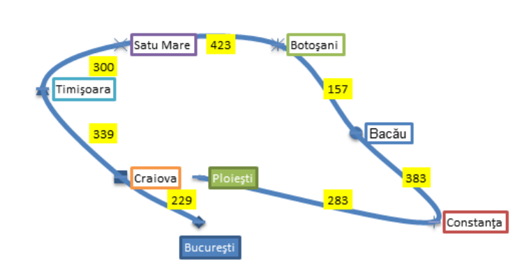
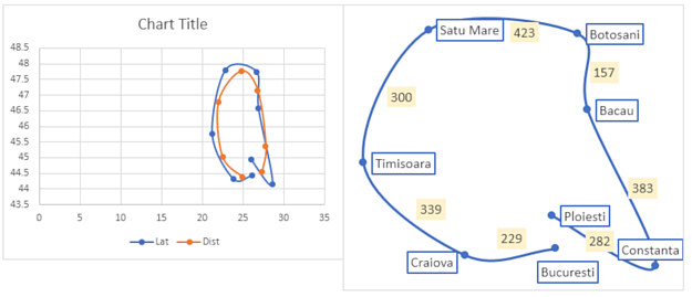
The plot on the left is the default chart; the one on the right is after formatting.

 

[alexdodo]

The exercised should be solved using Excel 2010.
Maybe with Diagram X/Y?

 

[mole999]

as you say, its an exercise, which is about putting into a test what you have learned. If being shown a way in 2013 that you HAVE to learn and know in 2010 then there is a gap in your knowledge YOU need to address

 

[alexdodo]

After some days, I did it using X/Y Diagram.

where alt_x is the average between x 1 and x 2(3 and 2) ...
and alt_y si the average between y 1 and y 2(1;2)....

Thanks boys.