On a matrix: If cells are marked, show table header value in corresponding row (with line breaks).

Chuck Rittersdorf

New Member
Joined
May 14, 2018
Messages
7
What is the best way to do the following:

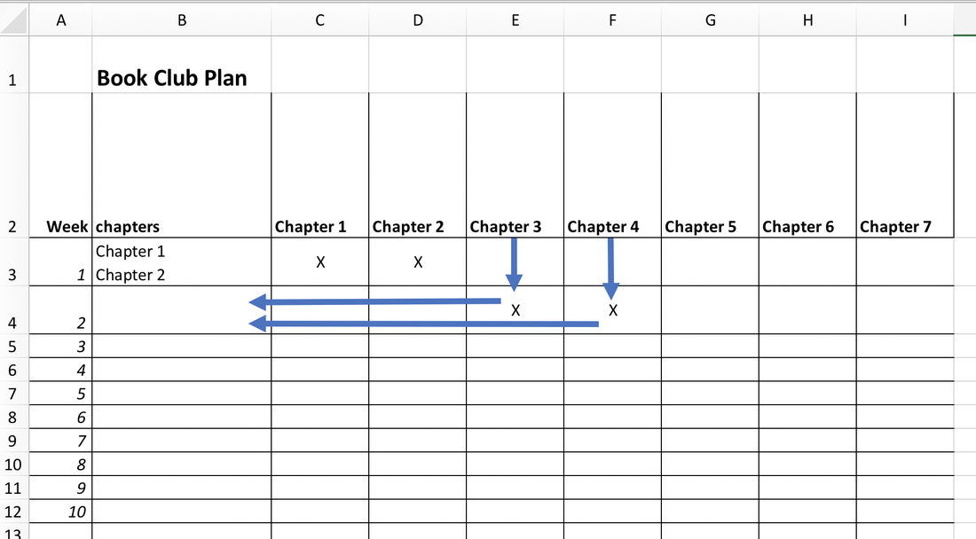
If one (or more cells) within a range on a matrix is marked (e.g. with "X"), show the value of the header in that column in the cell of the corresponding row left in the matrix (column B in my example).

If more than one cell (on a row) is marked, the values should be shown separated by a line break (on Mac and PC, I've heard there are issues).

Here is an image to explain what I mean:

problem_orig.png


I've tried an IF-function, but it does not accept ranges. I've considered Lookup, but my Excel-skills are too limited to use it... I'm working on a matrix with lots of rows and columns, so I need something copyable and hence time saving.

Please advice and thanks for your help.
 

Excel Facts

What is =ROMAN(40) in Excel?
The Roman numeral for 40 is XL. Bill "MrExcel" Jelen's 40th book was called MrExcel XL.
Welcome to the Board.

If you have one of the newer versions of Excel, then this would work in B3:

=TEXTJOIN(CHAR(10),TRUE,IF(C3:I3="x",C$2:I$2,""))
confirmed with Control+Shift+Enter. Change the ranges and copy down as needed.

Make sure that you have Word Wrap in your cells. If you don't have TEXTJOIN, then you'll need to use VBA in some way. Let us know.
 
Upvote 0
Thanks for your swift reply. Sadly my Excel 2016 for Mac does not have the function TEXTJOIN. Is there a similar function in my version? What would be a possible solution in VBA?

I have little experience with VBA, but I know a bit of Javascript. Should I start learning VBA and is it easy to pick up?
 
Upvote 0
TEXTJOIN is only available with an Office 365 subscription. There's a new version of Excel due later this year, so maybe that will have it.

If you have some programming experience, VBA is pretty easy to get into. But it's one of those languages that is very broad, there's a lot to learn. But much of that is specific to particular needs, so you may never need to learn it.

If you want to try a UDF (User-defined function), try this:

Open a copy of your workbook. Press Alt-F11 to open the VBA editor. From the menu, select Insert > Module. Paste this code into the window that opens:

Code:
Public Function MyConcat(ByVal MyHeaders As Range, ByVal MyData As Range) As String
Dim c As Long, h As Variant, d As Variant


    MyConcat = ""
    If MyHeaders.Rows.Count > 1 Or MyData.Rows.Count > 1 Or MyHeaders.Columns.Count <> MyData.Columns.Count Then
        MyConcat = "Invalid range size(s)"
        Exit Function
    End If
    h = MyHeaders.Value
    d = MyData.Value
    For c = 1 To UBound(h, 2)
        If LCase(d(1, c)) = "x" Then MyConcat = MyConcat & vbLf & h(1, c)
    Next c
    MyConcat = Mid(MyConcat, 2)
    
End Function
Now go back to your worksheet, and enter this formula in B3:
=MyConcat(C$2:I$2,C3:I3)

You can drag this down as needed. These instructions and code were designed on a Windows machine, if it doesn't work on your Mac, there's not much I can do. But I did steer clear of some things I know are not available on a Mac.

Let me know if you try this.
 
Upvote 0
Brilliant. That worked like a charm both on Mac and on PC. I had to make two little adjustments:
1. Turn the comma in =MyConcat(C$2:I$2,C3:I3) into a semicolon.
2. Turn "wrap text" on again.

You just saved me hours of work! Thanks again. Please let my know if I can do anything to thank you.
 
Upvote 0
One final question. Would it be possible to keep the source formatting with your vba-code? I found something about PasteSpecial. How do I plug it in?
 
Upvote 0
One final question. Would it be possible to keep the source formatting with your vba-code? I found something about PasteSpecial. How do I plug it in?

Sorry, I should never use the word final... Any way to make the row height auto/dynamic? Now I have to keep adjusting the row height manually with every change to see everything.
 
Upvote 0
First, a UDF returns a value only, no formatting. To change the formatting, you'd need a different type of macro. Maybe an event handler that triggers whenever you put an x in your data columns. But that depends on how those x's are entered.

As far as the row height, that little issue has bugged me for years! And a lot of other people, if Google is to be believed. I've written macros to try to figure out the right cell size, height and width to properly display something, but I never could. Font, line feeds, screen resolution, too many other factors to consider.

There is an option, AutoFit Row Height, but it's not dynamic. You can select the entire sheet by clicking on the upper left triangle (between the 1 and A). Then on the Home tab, Cells group, click Format > AutoFit Row Height. Voila! Every row is the right height. Until something changes. Then do it again. Not ideal, but the best I know. It could possibly be incorporated in another type of macro. Maybe someone else here has an idea. I'd like to know it myself!
 
Upvote 0
I see, formatting and functions don't go together...

About the auto row height: I found a way to reduce the number of steps. I made a button with this macro (see below). It ignores hidden stuff, which is handy. It's not superfast, but a lot faster than selecting all the rows and double click a row separator, which I was using before.

Code:
Sub refresh_rowheight()For Each rw In ActiveSheet.UsedRange.Rows
    If rw.Hidden = False Then
        rw.Range("A8:A625").EntireRow.AutoFit
    End If
Next
End Sub

The source of the complete macro (also with column height) is: https://www.experts-exchange.com/qu...there-are-hidden-rows-and-hidden-columns.html

Thanks once more!
 
Upvote 0

Forum statistics

Threads
1,214,649
Messages
6,120,733
Members
448,987
Latest member
marion_davis

We've detected that you are using an adblocker.

We have a great community of people providing Excel help here, but the hosting costs are enormous. You can help keep this site running by allowing ads on MrExcel.com.
Allow Ads at MrExcel

Which adblocker are you using?

Disable AdBlock

Follow these easy steps to disable AdBlock

1)Click on the icon in the browser’s toolbar.
2)Click on the icon in the browser’s toolbar.
2)Click on the "Pause on this site" option.
Go back

Disable AdBlock Plus

Follow these easy steps to disable AdBlock Plus

1)Click on the icon in the browser’s toolbar.
2)Click on the toggle to disable it for "mrexcel.com".
Go back

Disable uBlock Origin

Follow these easy steps to disable uBlock Origin

1)Click on the icon in the browser’s toolbar.
2)Click on the "Power" button.
3)Click on the "Refresh" button.
Go back

Disable uBlock

Follow these easy steps to disable uBlock

1)Click on the icon in the browser’s toolbar.
2)Click on the "Power" button.
3)Click on the "Refresh" button.
Go back
Back
Top