Help interpreting a formula Row(Indirect(A1&":"&A3))

ORoxo

Board Regular
Joined
Oct 30, 2016
Messages
149
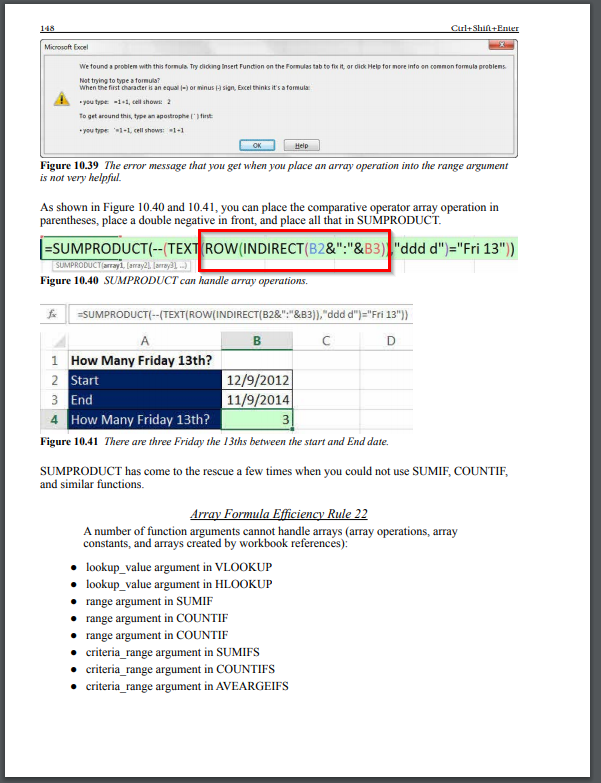
Guys, I have been reading Mike Garvins book - Ctrl+Shift+Enter Mastering Excel Array Formulas - and I am struggling to understand this specific part of the formula:
C7mXP3A.png


I understand that Row will return the rows of a given array. However, if INDIRECT returns serial number - which corresponds to dates - how can it extract the rows from it?

If you could shed light on this I would be extremelly grateful.
 
Last edited:

Excel Facts

Wildcard in VLOOKUP
Use =VLOOKUP("Apple*" to find apple, Apple, or applesauce
I understand that Row will return the rows of a given array. However, if INDIRECT returns serial number - which corresponds to dates - how can it extract the rows from it?

If you could shed light on this I would be extremelly grateful.
B2&":"&B3 forms the range 41252:41952 (if those are American dates) or the range 41164:41893 (if those are European dates). Let's stick with the American date assumption. When you wrap the ROW function around it, you get an array of row numbers, specifically, 41252, 41253, 41254, etc. and it is each one of those row numbers that is being fed into the TEXT function. But what are 41252, 41253, 41254, etc.? Why, they are date serial numbers for all the dates between the two dates specified in cells B2 and B3, so the formula ends up looking at each of these dates (via their date serial number) and formatting them as a three letter day name abbreviation followed by a space followed by a day number... it is this series of text values that are being compared to the constant "Fri 13" and, if any match, they are summed up via the SUMPRODUCT function call. Does that help you in understanding the formula any better?
 
Last edited:
Upvote 0
1. In Excel we can specify a row like this: 1:1. This means all of the cells of row 1. Again, 3:5, all of the cells from 3 to row 5 are implied. What we have here is a reference notation from a whole number to a whole number.

2. In

INDIRECT(1&":"&3)

with 1&":"&3 we get a text specification. The & operator creates a text result. Thus: "1:3" is what we get.

INDIRECT when fed with a text value like "1:3" tries to interpret it as a range.

3. If what INDIRECT looks at is a range, then the following is legal (legitimate)…

ROW(INDIRECT(4&":&7))

just like

ROW(A4:A7)

is.

4. ROW(range) delivers the row numbers of the cells composing the range.

Thus:

ROW(A4:A7) or ROW(INDIRECT(4&":"&7))

>>

{4;5;6;7}

5. A date value is a whole number.

When B2 and B3 houses dates, i.e. whole numbers:

B2&":"&B3 is text. Fed to INDIRECT, we get...

INDIRECT(B2&":"&B3)

This can be fed to ROW i.e.

ROW(INDIRECT(B2&":"&B3))

we get all of the dates between B2 and B3.
 
Upvote 0
B2&":"&B3 forms the range 41252:41952 (if those are American dates) or the range 41164:41893 (if those are European dates). Let's stick with the American date assumption. When you wrap the ROW function around it, you get an array of row numbers, specifically, 41252, 41253, 41254, etc. and it is each one of those row numbers that is being fed into the TEXT function. But what are 41252, 41253, 41254, etc.? Why, they are date serial numbers for all the dates between the two dates specified in cells B2 and B3, so the formula ends up looking at each of these dates (via their date serial number) and formatting them as a three letter day name abbreviation followed by a space followed by a day number... it is this series of text values that are being compared to the constant "Fri 13" and, if any match, they are summed up via the SUMPRODUCT function call. Does that help you in understanding the formula any better?

1. In Excel we can specify a row like this: 1:1. This means all of the cells of row 1. Again, 3:5, all of the cells from 3 to row 5 are implied. What we have here is a reference notation from a whole number to a whole number.

2. In

INDIRECT(1&":"&3)

with 1&":"&3 we get a text specification. The & operator creates a text result. Thus: "1:3" is what we get.

INDIRECT when fed with a text value like "1:3" tries to interpret it as a range.

3. If what INDIRECT looks at is a range, then the following is legal (legitimate)…

ROW(INDIRECT(4&":&7))

just like

ROW(A4:A7)

is.

4. ROW(range) delivers the row numbers of the cells composing the range.

Thus:

ROW(A4:A7) or ROW(INDIRECT(4&":"&7))

>>

{4;5;6;7}

5. A date value is a whole number.

When B2 and B3 houses dates, i.e. whole numbers:

B2&":"&B3 is text. Fed to INDIRECT, we get...

INDIRECT(B2&":"&B3)

This can be fed to ROW i.e.

ROW(INDIRECT(B2&":"&B3))

we get all of the dates between B2 and B3.

Guys, first of all, thank you both! It is quite clear now!

The only thing that bugs me is that when I try to evaluate the INDIRECT(B2&":"&B3) function through pressing F9 it gets me a range of 0 only. However, if I evaluate the whole formula - ROW(INDIRECT(B2&":"&B3)) - it works as supposed to

I was wondering why.

I do understand the complete formula now though!
 
Last edited:
Upvote 0

Forum statistics

Threads
1,214,523
Messages
6,120,028
Members
448,940
Latest member
mdusw

We've detected that you are using an adblocker.

We have a great community of people providing Excel help here, but the hosting costs are enormous. You can help keep this site running by allowing ads on MrExcel.com.
Allow Ads at MrExcel

Which adblocker are you using?

Disable AdBlock

Follow these easy steps to disable AdBlock

1)Click on the icon in the browser’s toolbar.
2)Click on the icon in the browser’s toolbar.
2)Click on the "Pause on this site" option.
Go back

Disable AdBlock Plus

Follow these easy steps to disable AdBlock Plus

1)Click on the icon in the browser’s toolbar.
2)Click on the toggle to disable it for "mrexcel.com".
Go back

Disable uBlock Origin

Follow these easy steps to disable uBlock Origin

1)Click on the icon in the browser’s toolbar.
2)Click on the "Power" button.
3)Click on the "Refresh" button.
Go back

Disable uBlock

Follow these easy steps to disable uBlock

1)Click on the icon in the browser’s toolbar.
2)Click on the "Power" button.
3)Click on the "Refresh" button.
Go back
Back
Top