COUNTIFS with MATCH INDEX (columns and rows)

[KrsOne20]

So I want to count the number of cells which are not blank or contain '-' in a range conditional based on column and row criteria. For example for firm 006 and period Q1-2011 I want to know the number of cells which are not empty or contain '-'. Answer should be 2.

For this purpose I want to combine COUNTIFS and MATCH INDEX formula. I have provided a screenshot of my data below (file is also included as attachment)

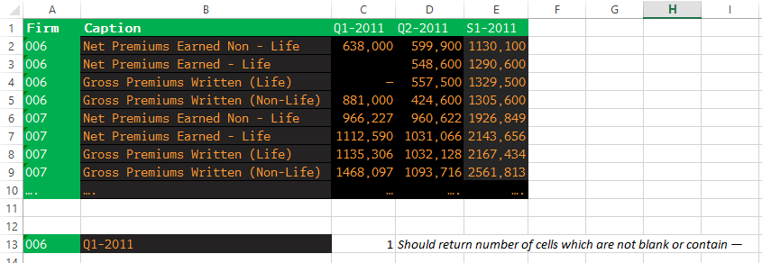
Im using this formula in cell C13, however it keeps returning 1. I think it doesnt look at the whole column but just at the first match of column/header.

=COUNTIFS(INDEX(A1:E10;MATCH(A13;A1:A10;0);MATCH(B13;A1:E1));"<>";INDEX(A1:E10;MATCH(A13;A1:A10;0);MATCH(B13;A1:E1));"<>—")

Anyone knows how I should adjust my formula? Thanks in advance!

Link to file: https://sheet.zoho.com/sheet/editor...762eed875098bf192d1a6a22ecbce1799f02eedfbf8f2

 

[sheetspread]

Excel 2010
	A	B	C	D	E
1	Firm	Caption	Q1-2011	Q2-2011	S1-2011
2	6	Net Premiums Earned Non - Life	638	599.9	1130.1
3	6	Net Premiums Earned - Life		548.6	1290.6
4	6	Gross Premiums Written (Life)		557.5	1329.5
5	6	Gross Premiums Written (Non-Life)	881	424.6	1305.6
6	7	Net Premiums Earned Non - Life	966.227	960.622	1926.85
7	7	Net Premiums Earned - Life	1112.59	1031.066	2143.66
8	7	Gross Premiums Written (Life)	1135.31	1032.128	2167.43
9	7	Gross Premiums Written (Non-Life)	1468.1	1093.716	2561.81
10	.	.		.	.
11
12
13	6	Q1-2011	2	Should return number of cells which are not blank or contain
Sheet18

Cell Formulas
Range	Formula
C13	=SUMPRODUCT(--($A$2:$A$9=A13)*--($C$1:$E$1=B13)*--(ISNUMBER($C$2:$E$9)))

works in your example, but there are no zeroes. If that's a problem I can change the formula.

 

[KrsOne20]

Excel 2010
.....
works in your example, but there are no zeroes. If that's a problem I can change the formula.

Thanks it works! The zeroes are not a issue as they are not present.

 

[KrsOne20]

After getting more into it, I have two minor observations (not a big deal, but maybe it can be fixed):

1) The weird thing is, for firms over #100 it doesn't work. Maybe due to the fact that the the firm number is stored as text (note: both data as my critera number is stored as text). 006 works fine, but 124 for example does not. In other formulas I have no issues looking up these firm numbers. However if I literally copy the number (e.g. 124) from the datasheet shown above and paste as my Lookup criteria it does work (but then the other lookup formulas dont work anymore)

2) Less important but just curious: Is this the only solution or is it still possible to do this with INDEX MATCH? The sumproduct seems quite heavy on the excel sheet (takes longer time to calculate), however Im not sure whether index match (or any other formula) would fix this.

 

[KrsOne20]

After getting more into it, I have two minor observations (not a big deal, but maybe it can be fixed):
1) The weird thing is, for firms over #100 it doesn't work. Maybe due to the fact that the the firm number is stored as text (note: both data as my critera number is stored as text). 006 works fine, but 124 for example does not. In other formulas I have no issues looking up these firm numbers. However if I literally copy the number (e.g. 124) from the datasheet shown above and paste as my Lookup criteria it does work (but then the other lookup formulas dont work anymore)

2) Less important but just curious: Is this the only solution or is it still possible to do this with INDEX MATCH? The sumproduct seems quite heavy on the excel sheet (takes longer time to calculate), however Im not sure whether index match (or any other formula) would fix this.

The 1st issue got solved by applying trim on the search criteria. For the 2nd if there is no better solution, I can just hardcode the values. But still curious if there is a alternative

 

[sheetspread]

Is this any faster?

Excel 2010
	A	B	C	D	E
1	Firm	Caption	Q1-2011	Q2-2011	S1-2011
2	6	Net Premiums Earned Non - Life	638	599.9	1130.1
3	6	Net Premiums Earned - Life		548.6	1290.6
4	6	Gross Premiums Written (Life)		557.5	1329.5
5	6	Gross Premiums Written (Non-Life)	881	424.6	1305.6
6	7	Net Premiums Earned Non - Life	966.227	960.622	1926.85
7	7	Net Premiums Earned - Life	1112.59	1031.066	2143.66
8	7	Gross Premiums Written (Life)	1135.31	1032.128	2167.43
9	7	Gross Premiums Written (Non-Life)	1468.1	1093.716	2561.81
10	.	.		.	.
11
12
13	6	Q1-2011	2	Should return number of cells which are not blank or contain
Sheet18

Cell Formulas
Range	Formula
C13	=COUNTIFS($A$2:$A$9,A13,INDEX($C$2:$E$9,,MATCH($B$13,$C$1:$E$1,0)),">=0")

It assumes positive numbers (otherwise there are workarounds)

You can convert numbers stored as text (common when importing from a database) by typing 1 in an unused cell, then copy-paste special-multiply to the range. Or a single line of VBA code. Don't just look at the format though to determine which is which, use the istext/isnumber functions.

 

[KrsOne20]

Is this any faster?
..

Thanks that defintely made it faster! I also have negative numbers. The workaround I did is the formula below (not the most fancy method, I just added another COUNTIFS to it). Is this the most efficient? Performance is still good tho.

=COUNTIFS([COLOR=Blue]$A$2:$A$9,A13,INDEX([COLOR=Red]$C$2:$E$9,,MATCH([COLOR=Green]$B$13,$C$1:$E$1,0[/COLOR])[/COLOR]),">=0"[/COLOR])+COUNTIFS([COLOR=Blue]$A$2:$A$9,A13,INDEX([COLOR=Red]$C$2:$E$9,,MATCH([COLOR=Green]$B$13,$C$1:$E$1,0[/COLOR])[/COLOR]),"<0"[/COLOR])

 

[sheetspread]

Try

=SUM(COUNTIFS($A$2:$A$9,A13,INDEX($C$2:$E$9,,MATCH($B$13,$C$1:$E$1,0)),{"<0",">=0"}))

 

[KrsOne20]

Try

=SUM(COUNTIFS($A$2:$A$9,A13,INDEX($C$2:$E$9,,MATCH($B$13,$C$1:$E$1,0)),{"<0",">=0"}))

Thanks, this is better