How to setup macro to reformat data

[jakeman]

Hi there - I'm not sure how to go about this problem. I have an existing table of data that is in a format which is not very usable. I want to reformat the data in a manner that requires a little bit of coding, otherwise I'll need to do data entry and that will take a long time.

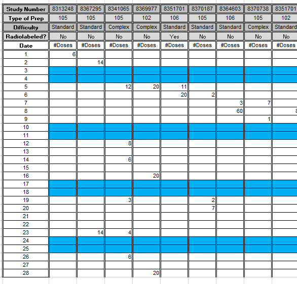
Currently my data is in this format:





However, I want to have the information in this format instead:



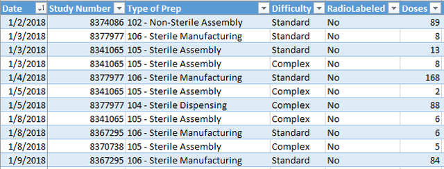
I am trying to create a macro that will step through each Study Number and as many entries there are for a month, to poplulate a table with the date, Study Number, Type of Prep, Difficulty, RadioLabeled, and finally the count. Essentially, this would be like a loop statement that will copy all of these fields for each Study until all dates have been copied, and then move on to the next study until all have been copied over.

Can anyone help with where to start with putting such a code statement together?

 

[tonyyy]

otherwise I'll need to do data entry and that will take a long time

While images are nice, it requires most anyone working on a solution "to do data entry..." You might get more responses if you post data that can be copied/pasted into excel.

Cheers,

tonyyy

 

[jakeman]

You're right! Here is the data in my existing format.

Study Number	10010	10020	10030
Type of Prep	32A	33B	32A
Difficulty	Standard	Complex	Complex
RadioLabeled?	No	No	Yes
Date	Doses	Doses	Doses
1/1/2018	4	5	18
1/2/2018	32	16	11
1/4/2018	15	11	10

<tbody>
</tbody>

Now I'd like it to be formatted to look like the following table:

Date	Study Number	Type of Prep	Difficulty	RadioLabeled	Doses
1/1/2018	10010	32A	Standard	No	4
1/2/2018	10010	32A	Standard	No	32
1/4/2018	10010	32A	Standard	No	15
1/1/2018	10020	33B	Complex	No	5
1/4/2018	10020	33B	Complex	No	11
1/2/2018	10030	32A	Complex	Yes	11
1/4/2018	10030	32A	Complex	Yes	10

<tbody>
</tbody>

 

[tonyyy]

jakeman,

Thanks for the data. You might consider the following...

Sub TransposeArray_1063501()
Dim LastRow As Long, LastCol As Long
Dim arr1 As Variant, arr2() As Variant
Dim newRows As Double
Dim r As Long, c As Long, i As Long

Application.ScreenUpdating = False
LastRow = ActiveSheet.Cells.Find(What:="*", after:=Cells(1, 1), LookIn:=xlFormulas, _
    LookAt:=xlPart, SearchOrder:=xlByRows, SearchDirection:=xlPrevious, MatchCase:=False).Row
LastCol = ActiveSheet.Cells.Find(What:="*", after:=Cells(1, 1), LookIn:=xlFormulas, _
    LookAt:=xlPart, SearchOrder:=xlByColumns, SearchDirection:=xlPrevious, MatchCase:=False).Column
arr1 = Range(Cells(1, 1), Cells(LastRow, LastCol))
newRows = WorksheetFunction.CountA(Range(Cells(6, 2), Cells(LastRow, LastCol)))
ReDim arr2(1 To newRows, 1 To 6)
i = 1

For r = 6 To UBound(arr1)
    For c = 2 To UBound(arr1, 2)
        If arr1(r, c) <> "" Then
            arr2(i, 1) = arr1(r, 1)
            arr2(i, 2) = arr1(1, c)
            arr2(i, 3) = arr1(2, c)
            arr2(i, 4) = arr1(3, c)
            arr2(i, 5) = arr1(4, c)
            arr2(i, 6) = arr1(r, c)
            i = i + 1
        End If
    Next c
Next r

Sheets.Add after:=Sheets(Sheets.Count)
With ActiveSheet
    .Range("A2:F" & newRows + 1).Value = arr2
    .Range("A1:F1").Value = Split("Date,Study Number,Type of Prep,Difficulty,RadioLabeled,Doses", ",")
    .Columns.AutoFit
End With
Application.ScreenUpdating = True
MsgBox "The dishes are done, dude!"
End Sub

Cheers,

tonyyy

 

[jakeman]

I'm going to try this out on the real thing but I gotta good feeling this will work, in which case my "dishes are done, man."

 

[jakeman]

Hey tonyyy - thanks for the code you supplied. I'm trying to adapt it to the exact scenario I need it for but I'm having some troubles that maybe you can help me with, if so inclined.

I have on one sheet 12 tables for each month, which I would like to individually copy/paste values from and paste to a consolidated table called YTD_Details. For now, I'm only concerned with transposing January data. The problem I'm having is that the table is creating several blank rows after the last row of data. Total number of rows in the table is equal to the newRows count, which in this case is 108. So from what I can tell, whenever cells within the newRows variable are blank, those becomes blank rows in my table. Don't know if you can try the code on your end and reproduce the issue. I'd sure be grateful if you could test it out.

Secondly, if there is already data in my table, ideally I would like to move to the next blank row and append data there. I don't think I understand your code well enough to figure out how to do that, but if you could explain what it's doing, maybe I could figure it out myself.

Thanks.

Sub TransposeArray_January()
Dim LastRow As Long, LastCol As Long
Dim arr1 As Variant, arr2() As Variant
Dim newRows As Double
Dim r As Long, c As Long, i As Long

Application.ScreenUpdating = False

LastRow = 39
LastCol = 21

arr1 = Range(Cells(4, 1), Cells(LastRow, LastCol)) 'Assigning the entire list of rows and columns that part of the range of cells needed to transpose to table

newRows = WorksheetFunction.CountA(Range(Cells(6, 2), Cells(LastRow, LastCol)))

ReDim arr2(1 To newRows, 1 To 6)

i = 1

For r = 6 To UBound(arr1)
    For c = 2 To UBound(arr1, 2)
        If arr1(r, c) <> "" Then
            arr2(i, 1) = arr1(r, 1)
            arr2(i, 2) = arr1(1, c)
            arr2(i, 3) = arr1(2, c)
            arr2(i, 4) = arr1(3, c)
            arr2(i, 5) = arr1(4, c)
            arr2(i, 6) = arr1(r, c)
            i = i + 1
        End If
    Next c
Next r

Sheets("Details").Select

N = Cells(Rows.Count, "A").End(xlUp).Row

With ActiveSheet
    .Range("A" & N & ":" & "F" & newRows + 1).Value = arr2
    .Columns.AutoFit
End With

Application.ScreenUpdating = True

End Sub

 

[tonyyy]

The problem I'm having is that the table is creating several blank rows after the last row of data. Total number of rows in the table is equal to the newRows count, which in this case is 108. So from what I can tell, whenever cells within the newRows variable are blank, those becomes blank rows in my table. Don't know if you can try the code on your end and reproduce the issue. I'd sure be grateful if you could test it out.

The code was tested against the sample data. If the sample isn't representative of the actual data then the results may differ.

That said, you're right to suspect the newRows variable...

newRows = WorksheetFunction.CountA(Range(Cells(6, 2), Cells(LastRow, LastCol)))

From the help file: The COUNTA function counts the number of cells that are not empty in a range. So newRows is the count of all the doses in Range(Cells(6,2), Cells(LastRow, LastCol)). If the Blank cells in the range are not blank, eg, if they contain a formula or other hidden text, then newRows will include those in the count... and the transformed data will include blank rows.

Let me know if this is indeed the case, then we can replace the newRows calculation with something else.

 

[jakeman]

Thanks, tonyyy. The sample data is representative of the actual data, it's just that the actual data contains more information and I had to adjust where the data begins and ends, that type of thing.

Let me just back up for one second and try to lay out what I'm trying to do. So your code works well when I use a table to transpose the data, but if I convert the table to a range, once data is transposed, the headers for the columns are wiped out. But for right now, I'm happy using a table actually.

But here is my dilemma. I want to be able to transpose data to my table but if there already exists data there, I want the information to be copied to the very next line. My problem right now is that this isn't happening and I've tried to code for that, but I can't seem to get it to work. Partly because I don't fully understand how your code works. Here is the code that I modified:

Sub TransposeArray_January()
Dim LastRow As Long, LastCol As Long
Dim arr1 As Variant, arr2() As Variant
Dim newRows As Double
Dim Rng As Range
Dim r As Long, c As Long, i As Long

Application.ScreenUpdating = False

LastRow = 39
LastCol = 21

arr1 = Range(Cells(4, 1), Cells(LastRow, LastCol)) 'Assigning the entire list of rows and columns that part of the range of cells needed to transpose to table

newRows = WorksheetFunction.CountA(Range(Cells(6, 2), Cells(LastRow, LastCol)))

ReDim arr2(1 To newRows, 1 To 6)

i = 1

For r = 6 To UBound(arr1)
    For c = 2 To UBound(arr1, 2)
        If arr1(r, c) <> "" Then
            arr2(i, 1) = arr1(r, 1)
            arr2(i, 2) = arr1(1, c)
            arr2(i, 3) = arr1(2, c)
            arr2(i, 4) = arr1(3, c)
            arr2(i, 5) = arr1(4, c)
            arr2(i, 6) = arr1(r, c)
            i = i + 1
        End If
    Next c
Next r

Sheets("Details").Select

N = Cells(Rows.Count, "B").End(xlUp).Row

With ActiveSheet
    .Range("B" & N & ":" & "G" & newRows + 1).Value = arr2
    .Columns.AutoFit
End With

On Error Resume Next
Set Rng = Range("YTD_Details[[Date]]").SpecialCells(xlCellTypeBlanks)
On Error GoTo 0
If Not Rng Is Nothing Then
    Rng.Delete Shift:=xlUp
End If

Application.ScreenUpdating = True

End Sub

Note that I hard-coded the values for LastRow and LastCol.

Also, variable "N" is meant to count the number of used cells in Column B of the Details sheet, which is where I want to copy and paste my data.

I appreciate your help, tonyyy.

 

[tonyyy]

Sub TransposeArray_January()
Dim LastRow As Long, LastCol As Long
Dim arr1 As Variant, arr2() As Variant
Dim newRows As Double
Dim Rng As Range
Dim r As Long, c As Long, i As Long, [COLOR=#ff0000]n As Long[/COLOR]

Application.ScreenUpdating = False

LastRow = 39
LastCol = 21

arr1 = Range(Cells(4, 1), Cells(LastRow, LastCol)) 'Assigning the entire list of rows and columns that part of the range of cells needed to transpose to table

newRows = WorksheetFunction.CountA(Range(Cells(6, 2), Cells(LastRow, LastCol)))

ReDim arr2(1 To newRows, 1 To 6)

i = 1

For r = 6 To UBound(arr1)
    For c = 2 To UBound(arr1, 2)
        If arr1(r, c) <> "" Then
            arr2(i, 1) = arr1(r, 1)
            arr2(i, 2) = arr1(1, c)
            arr2(i, 3) = arr1(2, c)
            arr2(i, 4) = arr1(3, c)
            arr2(i, 5) = arr1(4, c)
            arr2(i, 6) = arr1(r, c)
            i = i + 1
        End If
    Next c
Next r

Sheets("Details").Select

n = Cells(Rows.Count, "B").End(xlUp).Row
[COLOR=#ff0000]If Cells(n, 2) = "" Then
    n = Cells(Rows.Count, "B").End(xlUp).End(xlUp).Row + 1
Else
    n = Cells(Rows.Count, "B").End(xlUp).Row + 1
End If[/COLOR]

With ActiveSheet
    .Range("B" & n & ":" & "G" & newRows + 1).Value = arr2
    .Columns.AutoFit
End With

On Error Resume Next
Set Rng = Range("YTD_Details[[Date]]").SpecialCells(xlCellTypeBlanks)
On Error GoTo 0
If Not Rng Is Nothing Then
    Rng.Delete Shift:=xlUp
End If

Application.ScreenUpdating = True

End Sub

The .End(xlUp).Row will typically find the last row with data; when using a Table, however, it finds the last row in the Table, regardless if it contains data or not. The lines in red should account for this. (You may want to implement something similar where you have hard coded "LastRow = 39".

 

[jakeman]

I think this is working just fine for me now. Thanks for your help, tonyyy!

Just curious, did you build this code yourself or have you encountered this before?