Help w/SUMPRODUCT with Three Arrays/Conditions/AND

[GreganDunn]

I'm pretty sure that SUMPRODUCT is the solution to my problem here. I'm new to the SUMPRODUCT formula and fully understand it's basics and straight forward usage, however my SUMPRODUCT usage/requirement is a little more complex are I'm struggling with finding the right syntax to make things work for me.

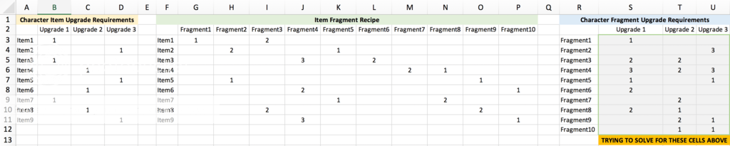
I'm attempting to create a new data set that lists the FRAGMENTS (or components) needed for a given UPGRADE based on the ITEM (items are composed of fragments) requirements for an upgrade and the RECIPE of the FRAGMENTS to create an ITEM.

I have an insane spreadsheet to plug this into, but I've narrowed it down and simplified it to the attached spreadsheet. The whole vertical/horizontal array thing is screwing me up in my specific example.

Thanks for taking the time to have a peak at my challenge, I really appreciate it!


Example File: https://www.dropbox.com/s/rqwq372hs2ome35/Upgrade Item to Fragments.xlsx?dl=0

Screenshot:

 

[Aladin Akyurek]

Instead of just "there it is and solve it", please try to help the helper...

Why is S5 2 if it is there where you need a formula?

 

[GreganDunn]

Of course I will try and help the helper, I gave as much information as I had and I'm here to help solve the problem.

I manually calculated the answers that I want in this simple set of data. My actual data set is MUCH larger and would be a severe amount of work to solve manually and I'd like the spreadsheet to be dynamic.

 

[Aladin Akyurek]

Of course I will try and help the helper, I gave as much information as I had and I'm here to help solve the problem.

I manually calculated the answers that I want in this simple set of data. My actual data set is MUCH larger and would be a severe amount of work to solve manually and I'd like the spreadsheet to be dynamic.

How does 2 of S5 obtain?

 

[sheetspread]

If you replace the blanks with zeroes:

Excel 2010
	R	S	T	U
1	Character Fragment Upgrade Requirements
2		Upgrade 1	Upgrade 2	Upgrade 3
3	Fragment1	1	0	0
4	Fragment2	0	0	3
5	Fragment3	2	2	0
6	Fragment4	3	2	3
7	Fragment5	1	0	1
8	Fragment6	2	0	0
9	Fragment7	0	2	0
10	Fragment8	2	1	0
11	Fragment9	0	2	1
12	Fragment10	0	1	1
13		TRYING TO SOLVE FOR THESE CELLS ABOVE
Sheet1 (2)

Cell Formulas
Range	Formula
S3:U12	{=MMULT(TRANSPOSE($G$3:$P$11),$B$3:$D$11)}
Press CTRL+SHIFT+ENTER to enter array formulas.

 

[sheetspread]

This works also as a single cell copied across/down without having to convert the blanks:

Excel 2010
	R	S	T	U
1	Character Fragment Upgrade Requirements
2		Upgrade 1	Upgrade 2	Upgrade 3
3	Fragment1	1	0	0
4	Fragment2	0	0	3
5	Fragment3	2	2	0
6	Fragment4	3	2	3
7	Fragment5	1	0	1
8	Fragment6	2	0	0
9	Fragment7	0	2	0
10	Fragment8	2	1	0
11	Fragment9	0	2	1
12	Fragment10	0	1	1
13		TRYING TO SOLVE FOR THESE CELLS ABOVE
Sheet1 (3)

Cell Formulas
Range	Formula
S3	=SUMPRODUCT(INDEX($G$3:$P$11,,ROW(A1)),INDEX($B$3:$D$11,,COLUMN(A1)))

or just =SUMPRODUCT(INDEX($G$3:$P$11,,ROW(A1)),B$3:B$11)

 

[GreganDunn]

This works also as a single cell copied across/down without having to convert the blanks:

Worksheet Formulas Cell Formula S3 =SUMPRODUCT(INDEX($G$3:$P$11,,ROW(A1)),INDEX($B$3:$D$11,,COLUMN(A1))) <thead> </thead><tbody> </tbody>

<tbody>
</tbody>

AMAZING! Totally works. Can you help me understand the logic that is taking place?

 

[GreganDunn]

Wish I could edit my posts to avoid multiple posts...

The question I have to help me understand this better, is how does the INDEX function refer to the "Upgrade", "Fragment" or "Item" columns as it's currently written? I.e how is it properly doing the multiplications?

 

[sheetspread]

You're just multiplying each fragment column by each upgrade column and finding the sum. The second table has fragments in a row instead of a column so you also have to transpose.

Index returns the nth column of the second table. You actually don't need it for the first table since the upgrade #s are already in columns. See the simpler formula I posted above: =SUMPRODUCT(INDEX($G$3:$P$11,,ROW(A1)),B$3:B$11)

 

[GreganDunn]

Awesome, thank you for the clarification. Now let's see if I can get this working in my beast of a spreadsheet...