minhhieule89
Board Regular
- Joined
- Jul 16, 2014
- Messages
- 68
Hi all, I have a spreadsheet like below
<colgroup><col span="3"><col span="2"></colgroup><tbody>
</tbody>
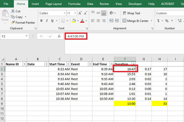
The Duration column is already calculated but I cannot use it since it's in the wrong format, when I sum the whole column I got 7:01 as the result which is not correct, the correct one should be 53 minutes
so I have to create helper column A which End Time minus Start Time, then helper column B which is taking HOUR(A)*60+MINUTE(A) to calculate in total how many minutes those event lasted
this is dump and I think there's must be a way to quickly calculate the 53 minutes, please help and thank you
| Start Time | End Time | Duration | A | B |
| 8:22 AM | 8:39 AM | 16:47 | 0:17 | 17 |
| 8:54 AM | 9:10 AM | 15:53 | 0:16 | 16 |
| 9:33 AM | 9:35 AM | 2:03 | 0:02 | 2 |
| 9:40 AM | 9:43 AM | 2:46 | 0:03 | 3 |
| 10:05 AM | 10:05 AM | 0:13 | 0:00 | 0 |
| 10:07 AM | 10:08 AM | 1:01 | 0:01 | 1 |
| 10:36 AM | 10:50 AM | 13:30 | 0:14 | 14 |
<colgroup><col span="3"><col span="2"></colgroup><tbody>
</tbody>
The Duration column is already calculated but I cannot use it since it's in the wrong format, when I sum the whole column I got 7:01 as the result which is not correct, the correct one should be 53 minutes
so I have to create helper column A which End Time minus Start Time, then helper column B which is taking HOUR(A)*60+MINUTE(A) to calculate in total how many minutes those event lasted
this is dump and I think there's must be a way to quickly calculate the 53 minutes, please help and thank you