Conditional format the top x non zero values by column

[John_Whin]

I don't know how to use an IF to select non zero values only for conditional formatting.

Ideally want to highlight the top x non zero values in column B only, then highlight top x non zero in column C only etc. Would like to do this across multiple columns.

Thanks

 

[Fluff]

Excel 2013/2016
	K	L	M
1	2	5	6
2	1	1	19
3	2	2	18
4	3	0	17
5	4	3	16
6	5	0	15
7	6	-1	14
8	7	-2	13
9	8	1	12
10	9	-4	11
11	10	-5	10
12	11	-6	9
13	12	-7	8
14	13	-8	7
15	14	-9	6
16	15	-10	5
17	16	-11	4
18	-17	-12	20
19	0	-13	20
20	0	-14	20
21	20	-15	3
22	21	-16	2
23	22	-17	1
Sheet1

Formula
=AND(K2 < > 0,(SUMPRODUCT(1-(K$2:K$20=0),--(K$2:K$20 > K2))+1) < =K$1)
Where K1, L1 & M1 are the number of values you want to highlight

 

[John_Whin]

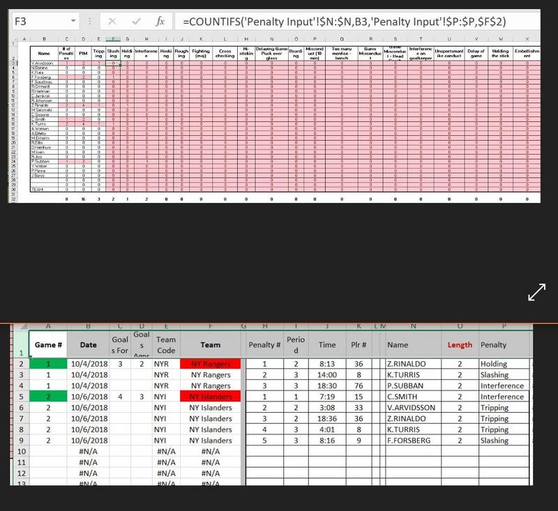
Thanks for trying to help, I'll be more specific. Making a hockey penalty spreadsheet and want to highlight the top 3 values in each column. Cells are loaded by function from data input throughout the season on Penalty Input sheet (see bottom image):

Example ... F3 has =COUNTIFS('Penalty Input'!$N:$N,B3,'Penalty Input'!$P:$P,$F$2) so it uses the players name to count the number of each penalty type that player gets as the season progresses.

I can Conditional Format to display the top 3 values in each column. But when the value is 0 as the table loads during the season there are lots of 0's that highlight as a top 3 value in that column.

So
I either need the Conditional Format to ignore the 0's on this sheet
or
I need an IF function that used the COUNTIFS as what is returned if condition is true and nothing (instead of 0) if the condition is false as it gets data from the Penalty Input sheet.

The IF functions I've tried return a 0 instead of a blank cell if the player has not committed that type of penalty.


maybe COUNTIFS isn't the right function choice in the first place.

tried to paste example but didn't work, how do I do that?

 

[Fluff]

As you may have noticed you cannot post images to the site.
If you just want the top 3 try
=AND(K2 < > 0,(SUMPRODUCT(1-(K$2:K$20=0),--(K$2:K$20 > K2))+1) < 4)

 

[John_Whin]

Here are a view of the sheets

 

[Fluff]

If I understand you correctly, the formula I supplied does what you are asking for.
Have you tried it?

 

[Peter_SSs]

If Fluff's solution is not what you need, can you tell us exactly what conditional formatting you have in cell C3 at the moment (assuming it does have CF applied)?

 

[John_Whin]

Actually I've got problems on several sheets in the same workbook this morning. On existing sheets even simple functions are not working. I've added a column for example.

in M13 I've got =K13. so I drag that simple formula up and down. (When I manually enter the =cellreference) it works fine. When I add a sheet and do same (even drag formula) it works OK.

But on existing sheets it is malfunctioning.

M11 contains =K11 but returns K13
M12 contains =K12 but returns K13
M13 contains =K13 and returns K13
M14 contains =K14 but returns K13
M15 contains =K15 but returns K13

First I did reopen the spreadsheet, did restart computer and did shut down and then start computer fresh.

[/IMG]

 

[John_Whin]

I did save as and reopen the new file, same problem

 

[Fluff]

As this is a completely different question to your OP, you'll need to start a new thread.

Also you never responded to either Peter or myself. Did you get your original question resolved?